Getting Started

1. Install and activate

System Requirement

The only mandatory requirement for using MiningMath is a 64-bits system, due to its use of Direct Block Scheduling technology. Other minimum requirements are listed further:

Windows 10
64-bits system (mandatory)
110 MB of space (installation) + additional space for your projects' files.
Processor: processors above 2.4 GHz are recommended to improve your experience.
Memory: at least 4 GB of RAM is required. 8 GB of RAM or higher is recommended to improve your experience.
Microsoft Excel.
OpenGL 3.2 or above. Discover yours by downloading and running the procedure available at here
Visual C++ Redistributable: Installation of Visual C++ Redistributable is necessary to run this software.

Recommended hardware

Memory should be a higher priority when choosing the machine in which MiningMath will be run on. In addition, a list of priority upgrades to improve performance with large scale datasets is given below.

Higher Ram
Higher Ram frequency
Higher processing clock

Installing

Installing MiningMath is quick and straightforward.. This guide will provide step-by-step instructions for installing the software on your computer.

Download the MiningMath Installer

Visit the MiningMath website at https://miningmath.com.
Click on the button located on the center of the homepage
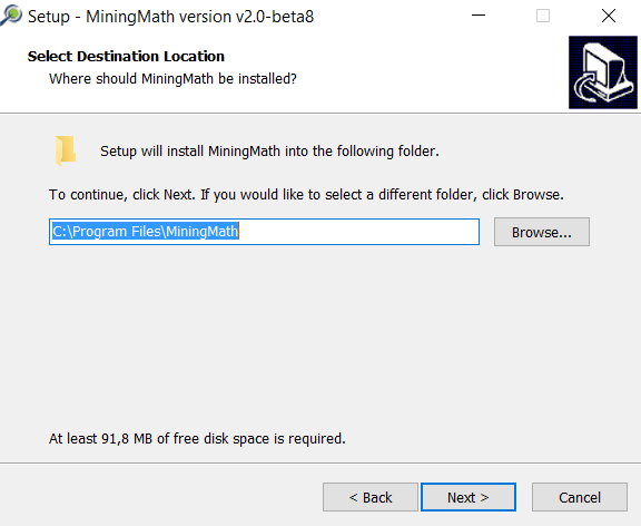
Save the installation file to your computer

Run the MiningMath Installer

Locate the downloaded installation file and double-click to launch the installer.
The installation wizard will start. Follow the simple instructions in the prompt until the installation has been completed.

Carefully read the license agreement before proceeding with the installation. If you agree to the terms of the agreement, click the "I accept the agreement" checkbox and then click the "Next" button.

Choose the location where you want to install the MiningMath software. If you wish to change the default location, click the "Browse" button to select a new folder and click "Next" to proceed.

Select any additional tasks you wish to perform during the installation process. Options include creating a desktop icon. Click "Next" to continue.

Review the installation settings before proceeding. If everything looks correct, click the "Install" button to begin the installation process.

The installer will start installing the MiningMath software on your computer. The progress bar will show the status of the installation.

Once the installation is complete, click the "Finish" button to exit the installation wizard. The MiningMath software is now installed on your computer.

Congratulations! You have successfully installed the MiningMath software on your computer.

Activating Your License

The free version of the MiningMath software is automatically activated upon installation and is valid for 60 days. After this period, it can be renewed for free by contacting MiningMath support.

To activate the full version of the software, follow these steps:

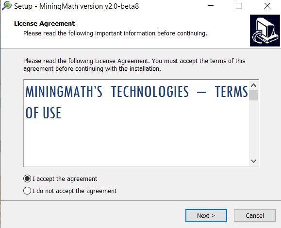
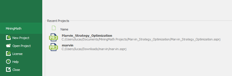
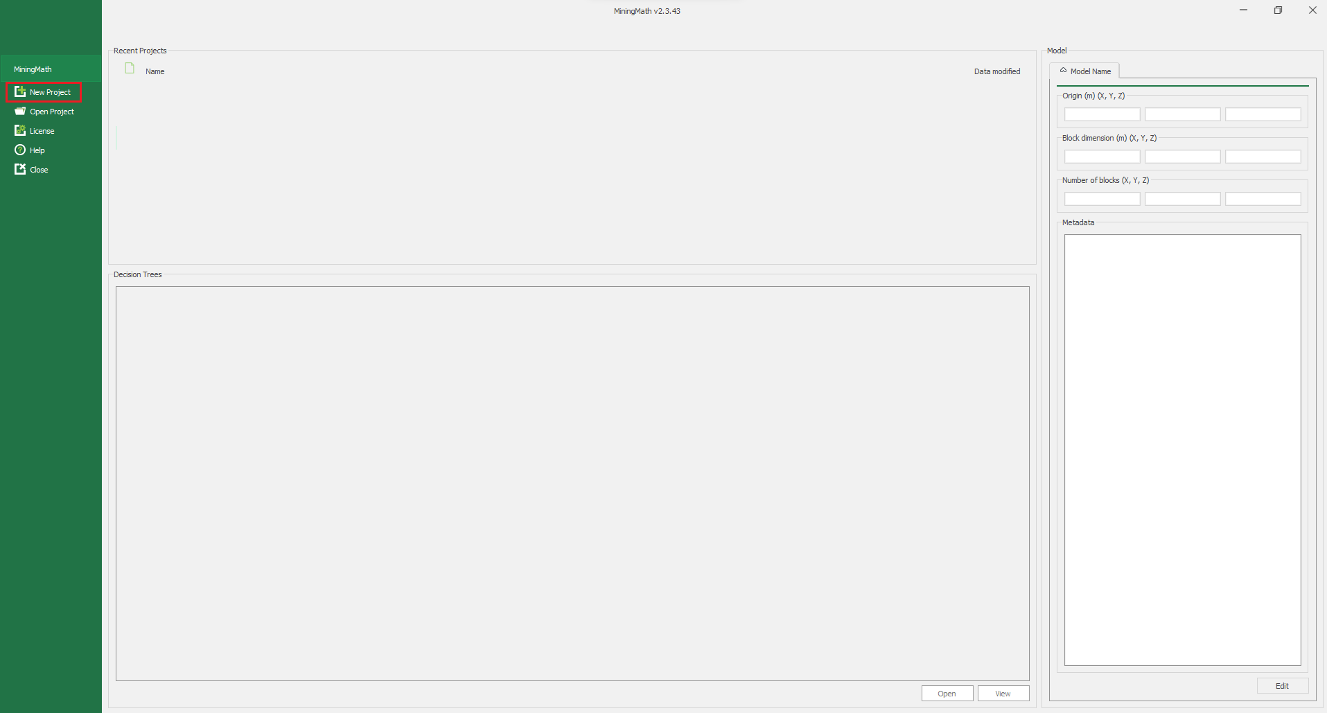
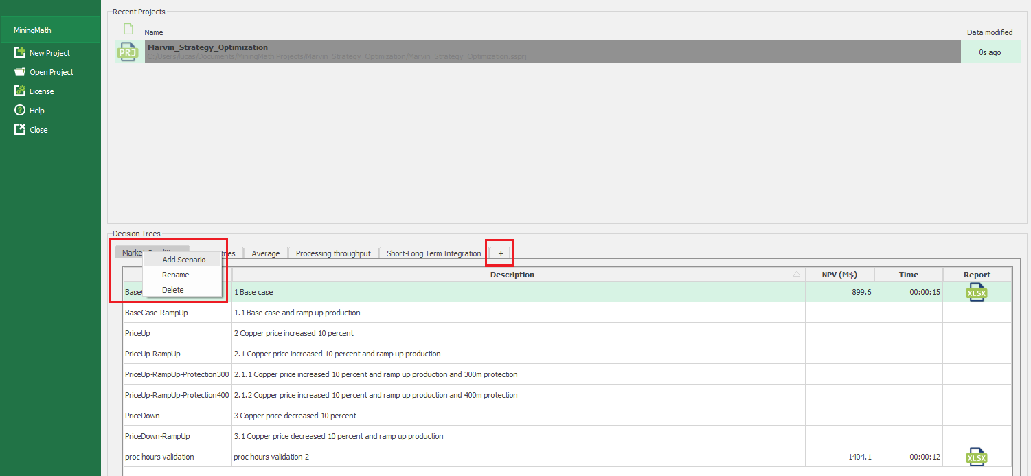
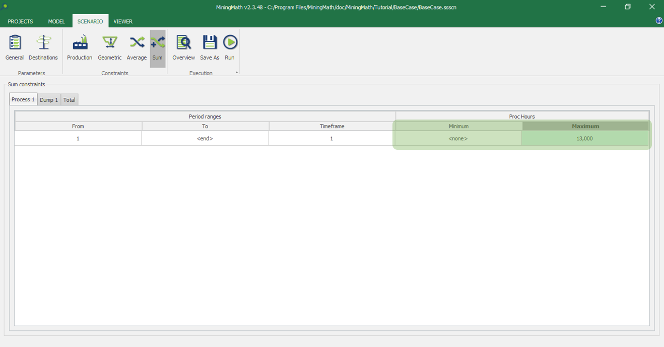
Open the MiningMath software and click on the "License" option in the left column.
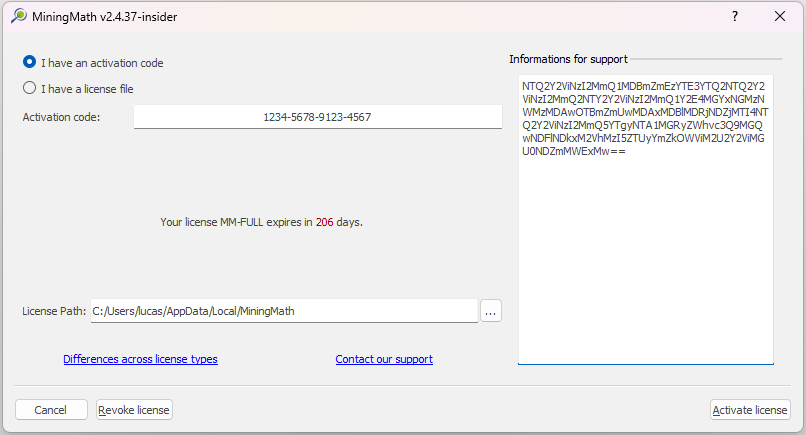
Enter your activation code into the field provided and click on "Activate License". Make sure that your computer is connected to the internet. The software will contact the activation server and complete the activation process.

Activation code

It is important to keep your activation code safe and secure, as it will be required in case you need to reinstall the software.

If you encounter any issues during the activation process, please contact MiningMath support for assistance.

2. Quick testing

The software comes with a pre-installed project called Marvin_Strategy_Optimization, which uses the Marvin deposit, a widely used dataset in the literature. This project contains various pre-configured scenarios that will be useful in the future to learn how to use the software.

Follow these steps to quickly test the software:

Select the Marvin_Strategy_Optimization project and save it to a folder on your machine where you have write permissions.
Once saved, double-click on the project to open it. This project contains several pre-configured scenarios that can be run to test the software.
Run some scenarios to familiarize yourself with the software's configuration, execution, and results process.

The Marvin deposit will also be used in the next steps of this guide.

3. Formatting stage

Note: the examples in this page are made with the Marvin dataset that comes pre-installed. Still, these steps would be the same if you were using your own data.

In order to use the software, you need to import your block model into the system. To do this, it is necessary to follow certain formatting specifications and assign the proper field types to each column of the block model.

Formatting Specifications

Regularized block model: All blocks must be the same size.
Air blocks must be removed prior to importation. This is the way MiningMath recognizes the topography.
Coordinates of each block in the 3 dimensions.
Header Names should not have special characters or have them exceed 13. Use this recommendation for folders and files also.
The data format should be a CSV file (Comma Separated Value), which might be compatible with most mining packages. An example can be seen below.

Good practices

Configure Microsoft Windows number formatting to use dot as the decimal separator.
Use the metric system.
Set multiple fields that will consider different economic values, material types, contaminant limits, and any other variable you wish to analyze or control.

Field types

Field Types are the fields MiningMath can understand. Each column imported should be assigned to the proper field type so that the software treats each variable accordingly with its meaning.

Mandatory Field Types

To run any optimization scenario, you will need to at least one field for each of these variables types:

Coordinates X, Y, and Z	Your geo-referenced information.
Average	Any variable that could be controlled by means of minimums and maximums considering its average: grades, haulage distance, and other variables.
Economic Value	Columns with the economic value when sent to the available destinations. It is possible to import multiple economic values at once, and they may be used simultaneously (ex.: multiple processing streams) or calculated in the internal calculator.

Optional Field Types

Density	Block's density.
Slope	Slopes varying block-by-block, which gives the flexibility to define slopes by lithotype and sectors
Recovery	Recoveries varying block-by-block.
Sum	Any variable that could be controlled by means of minimums and maximums considering its sum
Other	Information that you wish to have in the exported outputs
Skip	Any variable that should be ignored. This field type might help improve the runtime since these variables will not be considered and will not be exported along with the optimization outputs.

Software conventions

The model’s origin must be placed at the bottom portion

It should start to count from the minimum coordinates at X, Y, and Z (in this order). To clarify, the Z-coordinate grows first, followed by the Y-coordinate, and then the X-coordinate. In the Marvin example you can see how Z grows first for the same values of X and Y.

Note: Each software uses its own conventions for data format, naming, numbering systems, etc. These differences should be observed to prevent conflicts when working with data from multiple software.

What you must know

MiningMath uses coordinates (X,Y,Z) for which Z represents the elevation starting upwards

Other mining software may use indexes with IZ starting downwards. MineSight is an example that uses this notation.

To invert downwards coordinates use the following formula to convert: new(Z)=max(Z)+1–current(Z)

Air blocks

MiningMath recognizes that all imported blocks of your model are underground. This means it is necessary to remove all the air blocks prior to importation. Unless your topography is totally flat, which is unlikely.

The non-removal of air blocks may lead to unsatisfactory results and long processing times, since it would be considering blocks that do not exist in reality. The following video shows how to remove air blocks using filters on MS Excel. These tips are also applicable to any mining software of your choice.

Common issues

If you are having issues formatting your CSV check some common problems here. You can also post questions in our forum so the community can quickly help you.

4. Importing stage

Note: the examples in this page are made with the Marvin dataset that comes pre-installed. Still, these steps would be the same if you were using your own data.

To import the block model, select the option New Project on the left panel of MiningMath.

Afterwards, the file name input field is shown in red, indicating a mandatory field. Browse for and select the CSV formatted file. Press Next to advance.

After selecting the CSV file you should enter the Model Name. Optionally, the destination folder (Model Folder) can be changed as well as the Scenario Name, and a Scenario Description can be added.

Summary statistics

Upon clicking Next, the following window will provide a statistical summary of information for the block model that will be imported.

Coordinates

After importing the CSV file into MiningMath, you will need to specify the origin, and block dimensions. The number of blocks is automatically calculated based on this information. In this project, the origin was x=0, y=0, and z=0, and the block dimensions were 30 meters in each coordinate.

Column types

After clicking Next, a form appears, linking the imported CSV file headers to available field types in MiningMath. Each imported column must be associated with a corresponding field type, such as block coordinates with Coord. X, Y, and Z.

Other columns

Typically, MiningMath recognizes some columns automatically when their headers are similar to the field type name. Otherwise, MiningMath will automatically assign them to the field type Other.

Next buttom

To enable the Next button, you need to assign the coordinates and at least one other data column. MiningMath requires some mandatory fields to run a scenario, such as economic value for the processing plant and waste dump. If these are not defined now, you will be able to add them later using the internal calculator.

Grade units

After clicking Next, MiningMath will require grade units. In the Marvin example, the copper grade has been defined as a percentage (%), while gold grade was defined as PPM, which stands for parts per million and, in turn, is equivalent to g/ton.

View model

By clicking on View Model you will be able to visualize your data in the Viewer tab and do some preliminary evaluation. By clicking on Setup Scenario you will be redirected to the scenario tab to create your first scenario to be optimized.

You can have a quick look at your imported data in the Model tab. Don’t worry about checking every detail at this stage. You will have the chance to fully validate your data at the next steps.

5. Calculator stage

Note: Using the internal calculator is not a required step for creating scenarios and optimizing your model. It is only required if you don’t have economic values or if you need to derive new fields not present in the original data.

By using the calculator you can define new fields based on your imported values. Any calculation can be done in the Function tab.

Example

The most common use of the calculator is to create new economic values. You can learn more about destinations required in the explanation below.

MiningMath does not require pre-defined destinations ruled by an arbitrary cut-off grade. Instead, the software uses an economic value for each possible destination and for each block. The average grade that delineates whether blocks are classified as ore or waste will be a dynamic consequence of the optimization process.

Therefore, MiningMath requires at least two destinations: 1 processing stream and 1 waste dump. Therefore, each block must be associated with:

1 Economic value for the processing plant
1 Economic value for the waste dump

MiningMath can determine the best destination option during optimization without the user pre-setting it. If you don’t have economic values defined in your model, you can use the example below as a guide to calculate them.

Note: Even blocks of waste might have processing costs in the economic values of the plant. Therefore, non-profitable blocks would have higher costs when sent to process instead of waste.

Note: If you have any material that should be forbidden in the plant, you can use economic values to reduce the complexity and runtime, as mentioned here.

The definition of economic values involves considering factors such as the destination of the block, grades, recovery, mining cost, haul costs, treatment costs, blasting costs, and selling price.

An example of the calculation is provided with the calculation parameters listed below.

Description	Cu (%)	Au (PPM)
Recovery	0.88	0.6
Selling price (Cu: $/t, Au: $/gram)	2000	12
Selling cost (Cu: $/t, Au: $/gram)	720	0.2
Processing cost ($/t)	4
Mining cost ($/t)	0.9
Discount rate (%)	10
Dimensions of the blocks in X, Y, Z (m)	30, 30, 30

Block Tonnes

Block Tonnes = BlockVolume * BlockDensity
Block Tonnes = 30*30*30*[Density]

Tonnes Cu

Tonnes Cu = Block Tonnes x (Grade Cu/100)
Tonnes Cu = [BlockTonnes]*([CU]/100)

Mass Au

Mass Au = Block Tonnes x Grade Au
Mass Au = [BlockTonnes]*[AU]

Economic Value Process

Economic Value Process =
[Tonnes Cu x Recovery Cu x (Selling Price Cu – Selling Cost Cu)] +
[Mass Au x Recovery Au x (Selling Price Au – Selling Cost Au)] –
[Block Tonnes x (Processing Cost + Mining Cost)]
Economic Value Process = ([TonnesCu]* 0.88 * (2000–720)) + ([MassAu] * 0.60 * (12 – 0.2)) – ([BlockTonnes] * (4.00 + 0.90))

Economic Value Waste

Economic Value Waste = –Block Tonnes x Mining Cost
Economic Value Waste = –[BlockTonnes] * 0.9

The block in the example above would generate -299,880$ if sent to the process, and –55,080.1$ if discarded as waste. Therefore, this block might go to waste, since it would result in less loss than when it is processed. MiningMath defines the best destination regarding the set of constraints throughout the time, thus this decision is a lot more complex than the example above in most cases.

Tip: You can use the calculator to define multiple economic values. For example, what if the selling price or selling cost of Cu varies? These alternative scenarios can be evaluated later on with the help of our decision tree. To learn more about the calculator click here.

6. Validation stage

Complex projects with many constraints may demand hours to execute. Hence, it is important that imported data is validated before to avoid possible errors. This page provides an example with the Marvin Deposit and shows how you can set up and run a scenario to validate your data.

Set up

In order to validate your data and make sure there are no apparent errors in it, the following setup is recommended:

Process and dumps set with respective recovery values.
A bigger production capacity than the expected reserves. In this example, the expected life of mine vs production rate is 35-year producing 10 Mt per year. Hence, a value of 1,000 Mt would be big enough to cover the whole reserve.
No discount rate.
No stockpiling.
Density and slope values.
Timeframe: Years (1), since it would all be processed in 1 period.

You can create a new scenario by right clicking in a decision tree. If you don’t have any decision trees, you can create one by clicking on the + sign.

After creating a scenario, you will be prompted to enter general parameters, such as density and slope angles.

The Destinations tab should be enabled after entering the general parameters.

Here, you need to add at least one process and one waste dump.

Next, you will be required to add the Production limits.

For the Validation scenario, you can use years in the Timeframe and an unbounded value for the process, for example 1,000,000,000.

The Overview tab will give you a general view of your setup. For the Marvin dataset, the validation will be as depicted below.

Lastly, you can run the scenario by using the Run button at the top.

Results

Once the execution has finished, you will be able to visualize the reports in the same tab, or open the respective csv and xlsx files in Excel. This execution will also generate the topography surface that you can as an example to create other surfaces, for instance force or restrict mining areas. After running the suggested scenario, you should evaluate the results in the Viewer tab and the respective reports in Excel.

Evaluation

Evaluating the results reported in the validation should help you identify any apparent problems that you can fix before running more complex scenarios. Some of the common questions that might help you in this analysis:

Did the scenario run properly?
Are most of the positive economic values from the process inside this surface?
Is the mining happening in reasonable areas?
Is the NPV reported reasonable for an unrestricted scenario?

If your validation does not seem correct, you might have to reevaluate your block model. For example, there might be wrong values in the data imported, errors with data formatting, or if you used the internal calculator, there might be something wrong with the formulas applied. Otherwise, if everything seems correct, you should proceed to the next page.

7. NPV upper bound

Before adding more complex constraints to your project, it is important to have some general idea of how high the NPV of your project can be. The NPV upper bound is an unrealistic limit, but it can help as a reference point as you progress through the project and add all its constraints at different steps.

At this stage, you can add some surface representing any restricted area in the project. Learn more about force or restrict mining areas. For the Marvin example there is no such restriction. However, if you are using your own data set, make sure that your surface files are well formatted as detailed here. You can use any previously generated surface, such as the topography, as an initial example to help you in this process.

You can run a scenario similar to the validation one including any force or restricted mining areas. The figure below shows an illustrative setup.

Super Best Case

The Super Best Case is the recommended approach to define the NPV upper bound. It aims to maximize the discounted cash flow of a project by exploring the entire solution space, with the only constraint being processing capacity. It is a global, multi-period optimization that seeks to uncover the full upside potential for the project’s net present value.

Set up

For the Marvin dataset, you can setup the Super Best Case similarly to the validation stage, but including the limit for processing capacity, which in this case is 30Mt per year.

Results

After running the Super Best Case scenario evaluate the results. You can check if restrictions are respected and if results in the report are reasonable.

Tip: It is important to mention that if you have multiple destinations, extra processing, or dump routes, it could be added for proper destination optimization (note that MiningMath does not apply the concept of cut-off grades). Besides that, the surfaces obtained here could be used in further steps or imported back into any mining package for pushback design and scheduling

8. Refining the NPV upper bound

After having identified the NPV upper bound of your project, it is recommended that you start adding average constraints, sum constraints, and stockpiling. If there are any average and sum variables in your project, they will be already imported at this stage. Nonetheless, you can always define new variables in the calculator if necessary. Next, you can see some examples of average constraints, sum constraints, and stockpiling being employed in the Marvin dataset.

Average constraints

Average constraints are based on quantifiable parameters modeled block by block. To use this feature, the dataset must include an auxiliary field/column representing the desired limit for each block.

When to use?

Average constraints are usually employed for blending low-grade and high-grade blocks to enhance profitability. Nonetheless, they have a diverse range of applications, being applicable to any variable that can be modeled based on these assumptions.

Set up

The figures below depict two parameters imported as average variables.

The limits of average variables can be defined in the Scenario tab. As depicted below, it is possible to input limits (A), for each period range (B), weights (C) and each destination (D).

You in Overview tab you can see these limits as depicted below.