if (typeof (wpDataCharts) == 'undefined') wpDataCharts = {};
wpDataCharts[2] = {
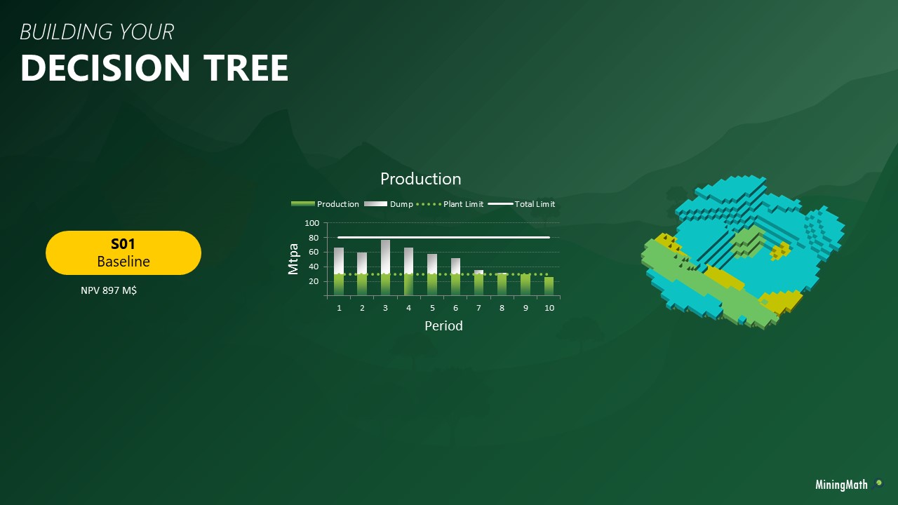
render_data: {"columns":[{"type":"number","label":"Period","orig_header":"Period"},{"type":"number","label":"Production Base Case","orig_header":"Production Base Case"},{"type":"number","label":"Production PriceUp","orig_header":"Production PriceUp"}],"rows":[[1,55.35,59.72],[2,51.8,66.84],[3,74.07,71.56],[4,68.69,76.52],[5,68.32,61.5],[6,42.18,44.34],[7,38.78,45.32],[8,30.69,55.43],[9,31.1,32.63],[10,16.24,30.19],[11,0,21.52]],"axes":{"major":{"type":"number","label":"Period"},"minor":{"type":"number","label":""}},"options":{"title":"Production PriceUp","series":[{"color":"#3366CC","label":"Production Base Case"},{"color":"#DC3912","label":"Production PriceUp"}],"height":400,"responsive_width":1,"hAxis":{"title":"Period","direction":"1"},"vAxis":{"title":"Tonnage (Mt)","direction":"1","viewWindow":{"min":"","max":""}},"backgroundColor":{"fill":"","strokeWidth":0,"stroke":"","rx":0},"chartArea":{"backgroundColor":{"fill":"","strokeWidth":0,"stroke":""}},"fontSize":"","fontName":"Arial","colors":["#3366CC","#DC3912","#FF9900","#109618","#990099","#3B3EAC","#0099C6","#DD4477","#66AA00","#B82E2E","#316395","#994499","#22AA99","#AAAA11","#6633CC","#E67300","#8B0707","#329262","#5574A6","#3B3EAC"],"curveType":"none","crosshair":{"trigger":"","orientation":""},"orientation":"horizontal","titlePosition":"out","tooltip":{"trigger":"focus"},"legend":{"position":"bottom","alignment":"end"}},"vAxis":[],"hAxis":[],"errors":[],"series":[{"label":"Production Base Case","color":"#3366CC","orig_header":"Production Base Case"},{"label":"Production PriceUp","color":"#DC3912","orig_header":"Production PriceUp"}],"group_chart":false,"show_grid":true,"type":"google_line_chart"},
engine: "google",
type: "google_line_chart",
title: "Production PriceUp",
container: "wpDataChart_2",
follow_filtering: 0,
wpdatatable_id: 4,
group_chart: 0 }

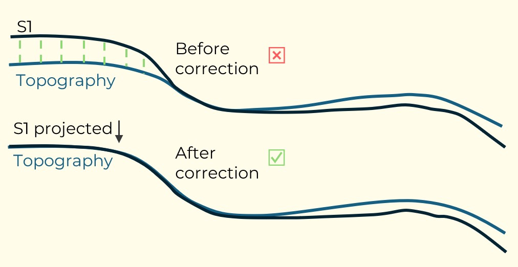
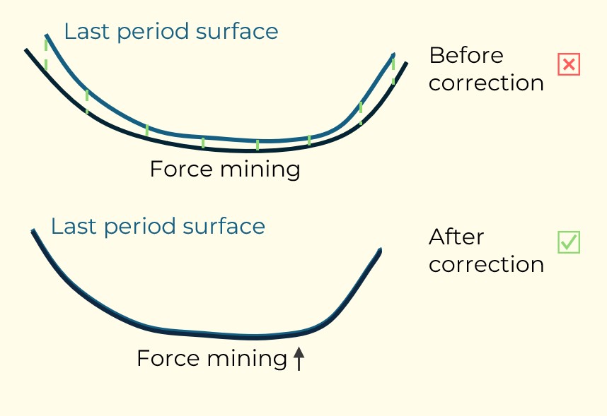
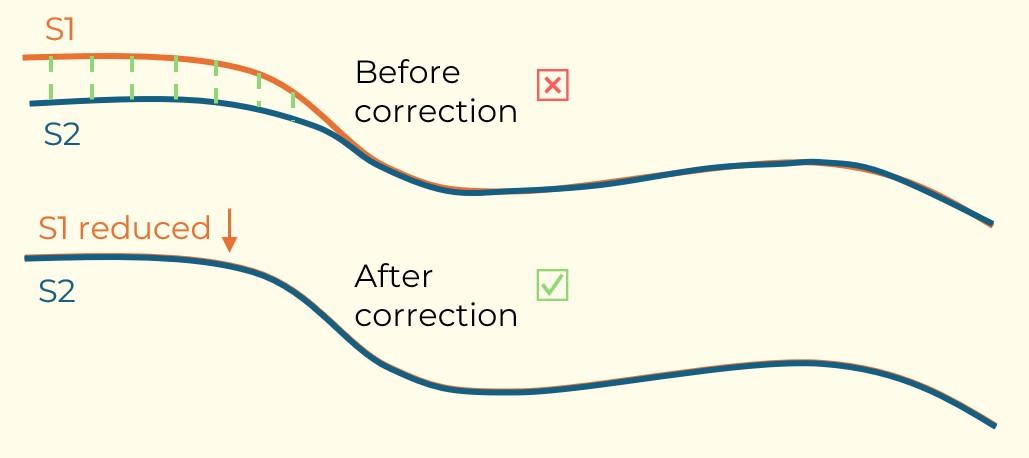
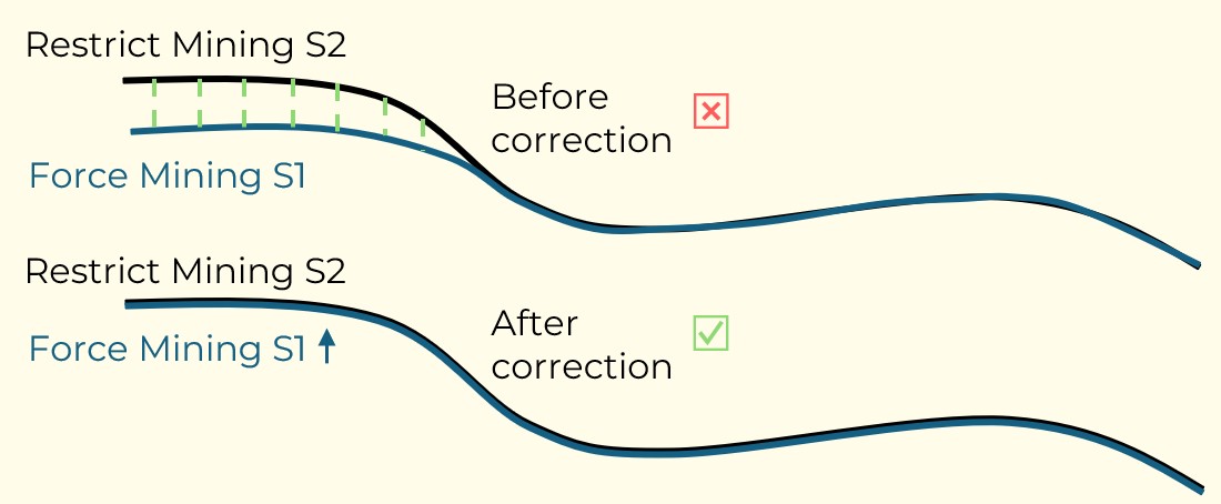
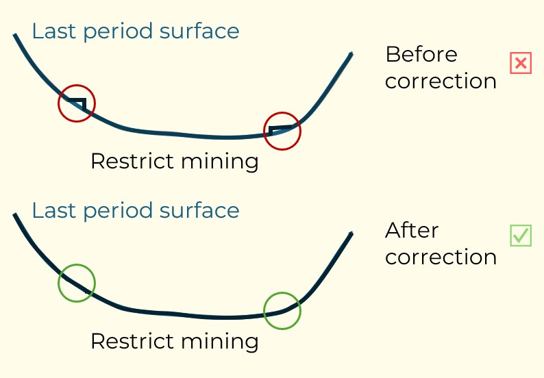
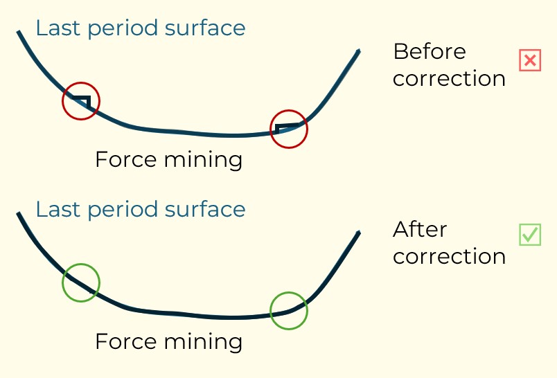
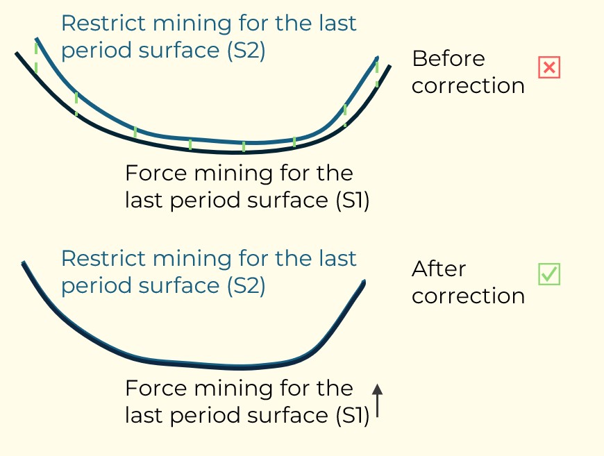
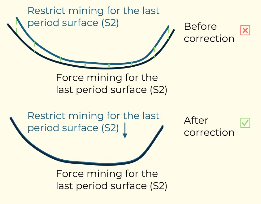
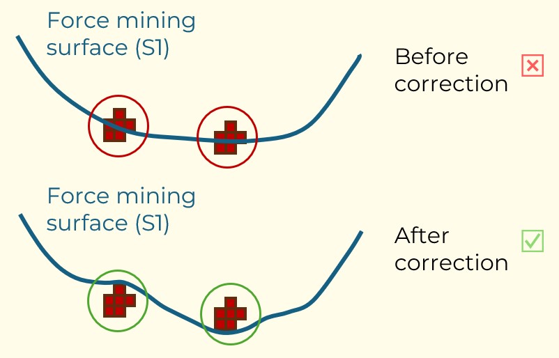
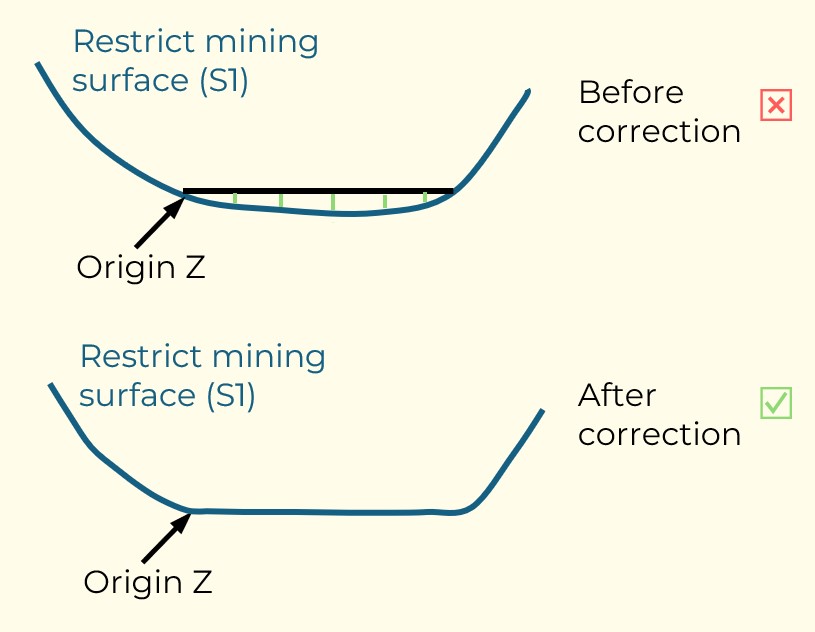
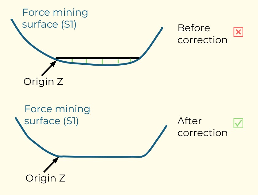
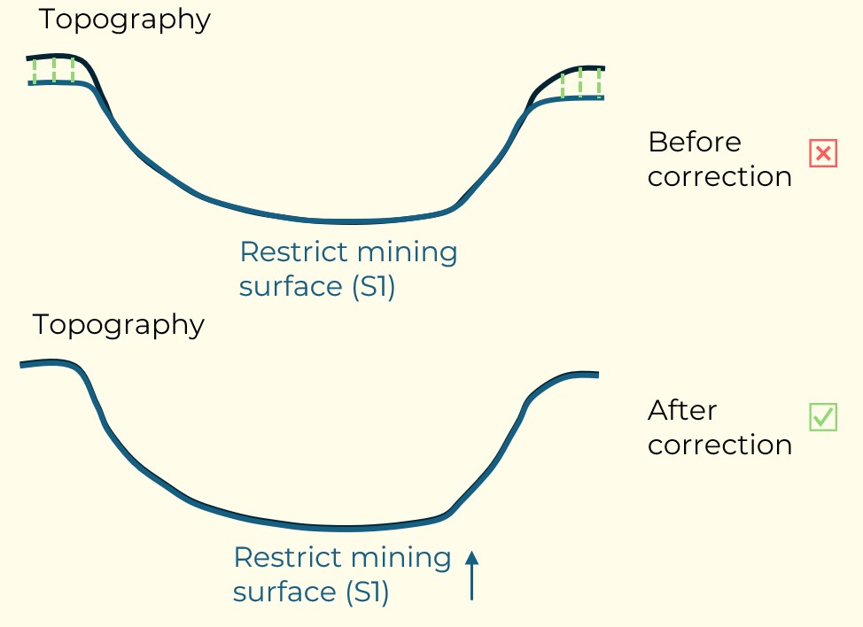
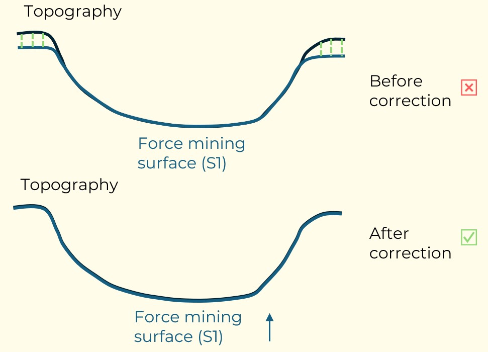
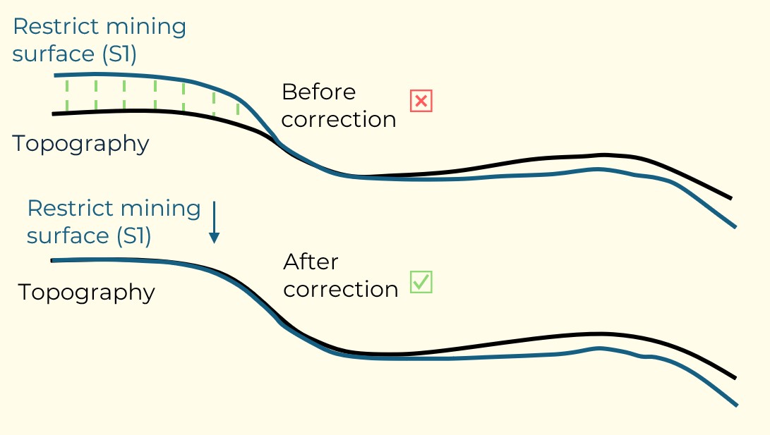
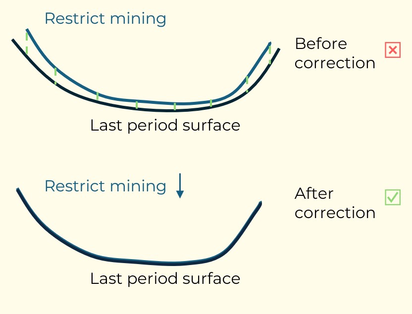
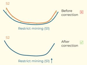
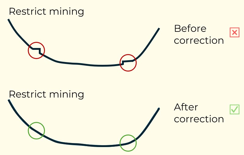
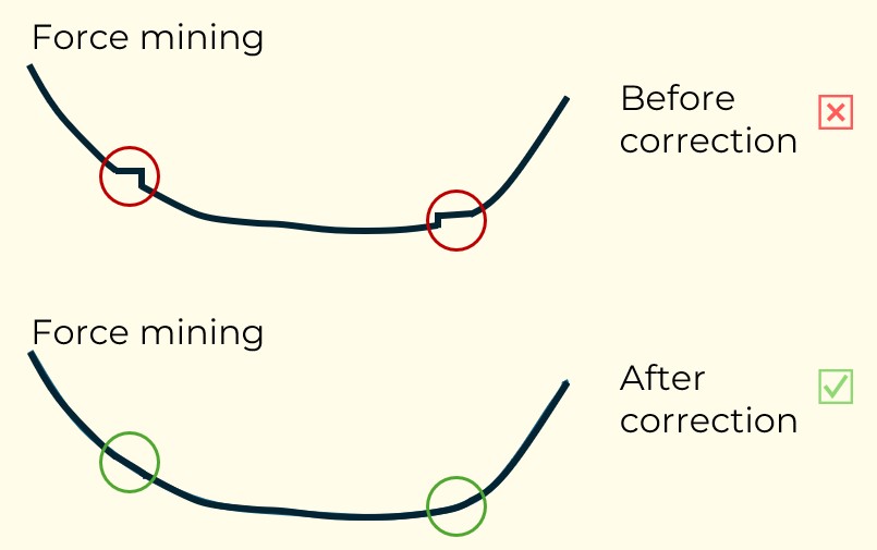

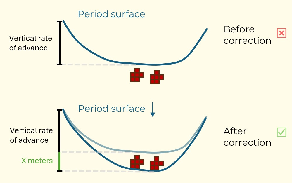


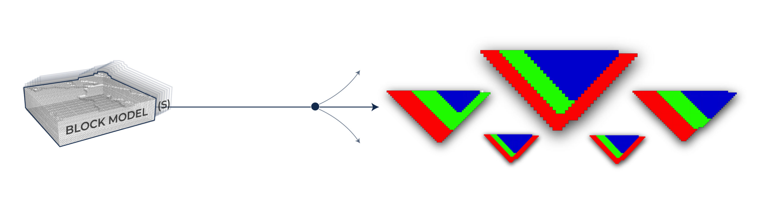
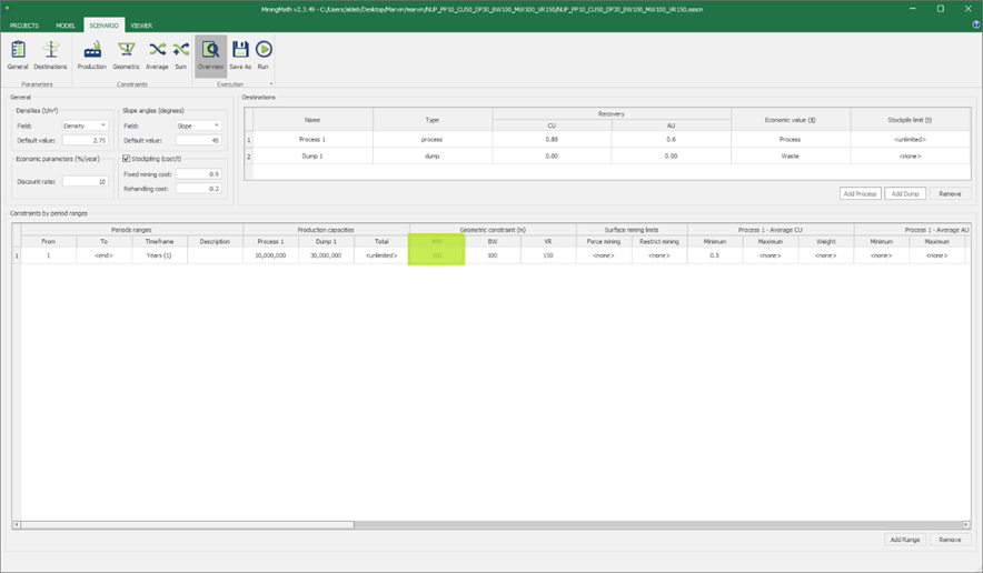


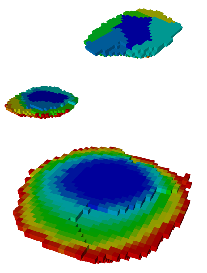

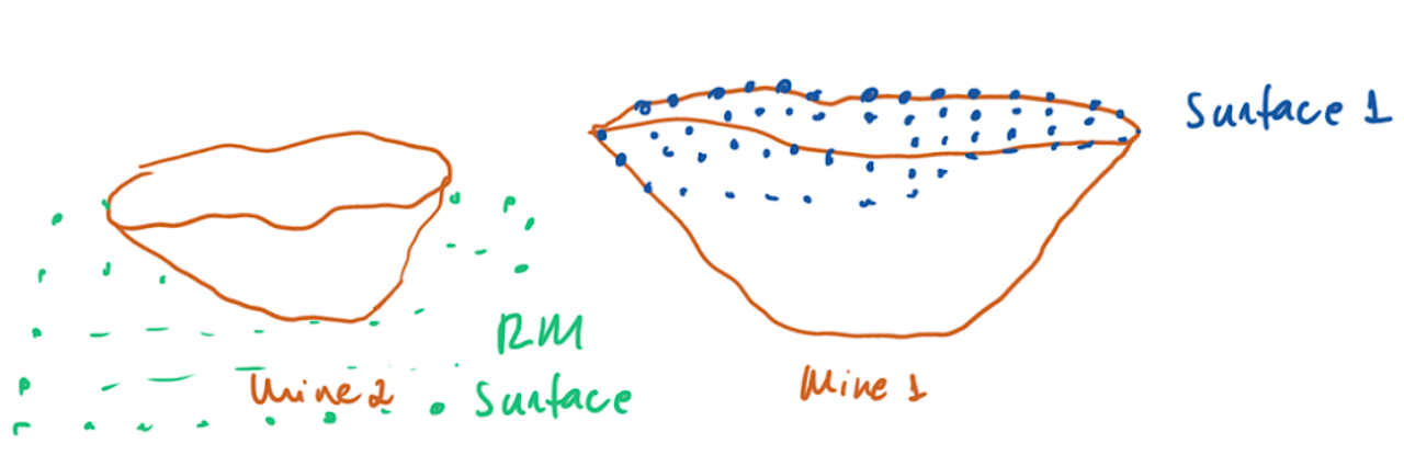
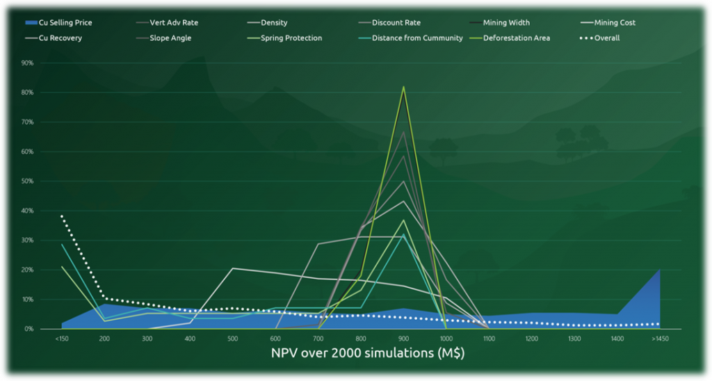
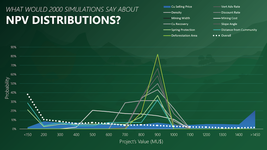
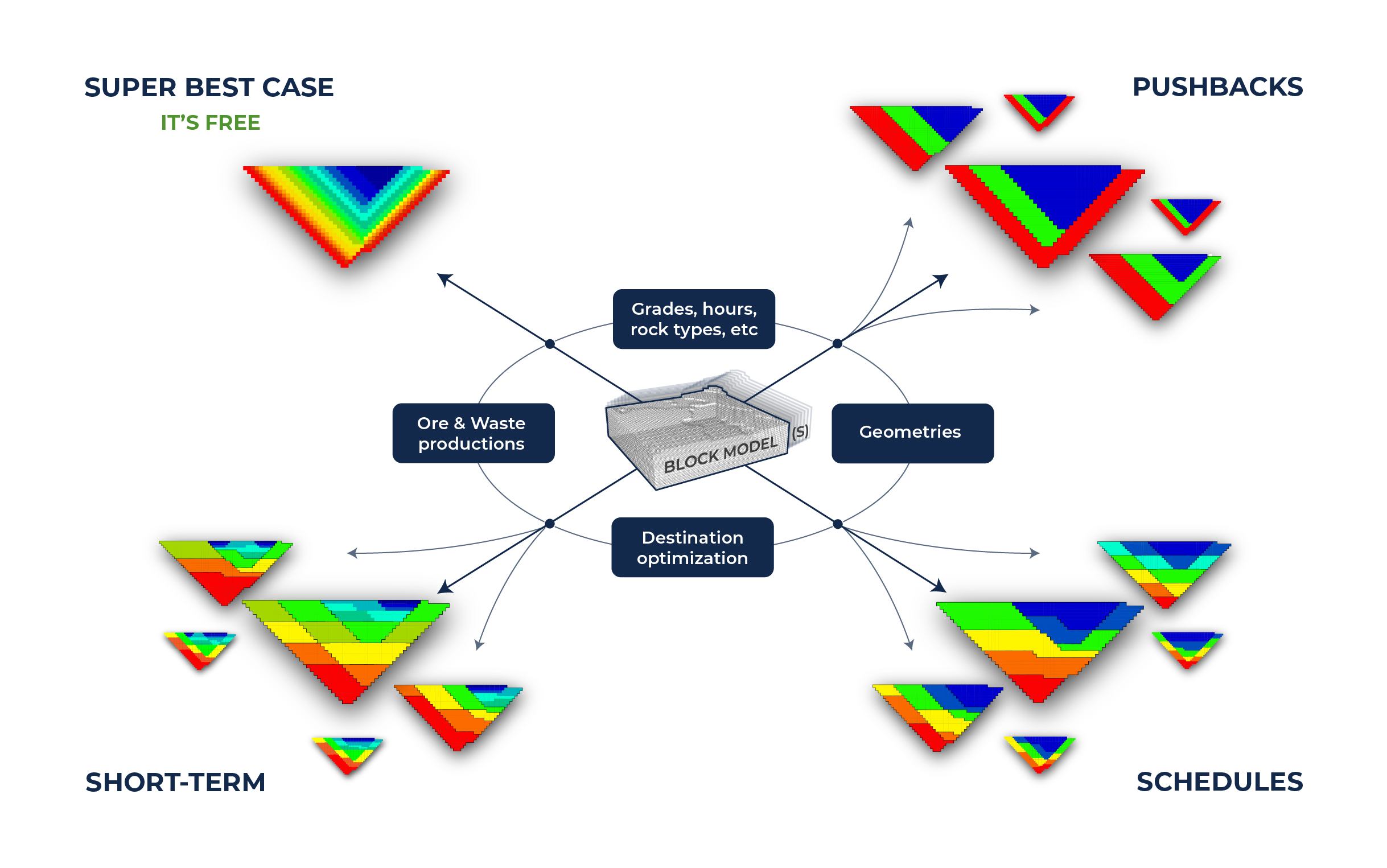
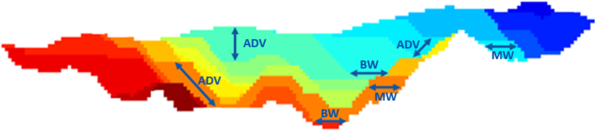
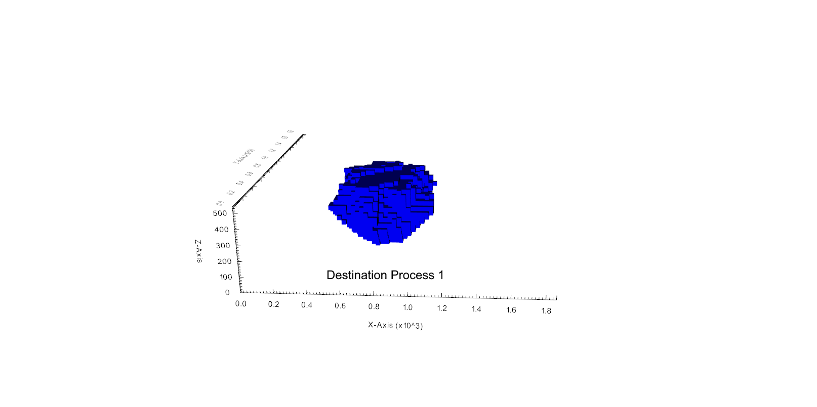
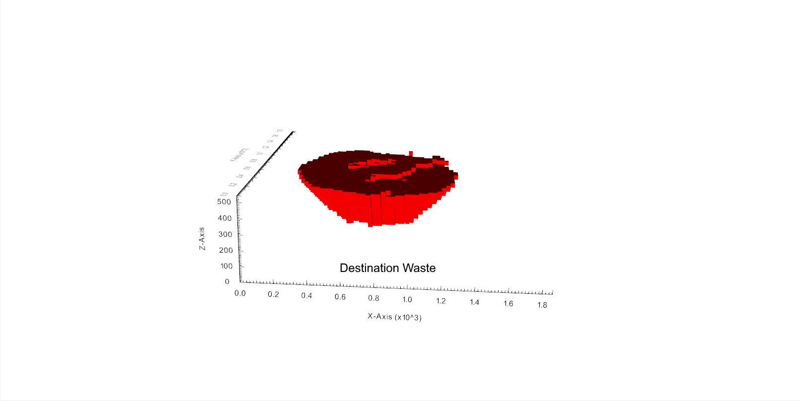
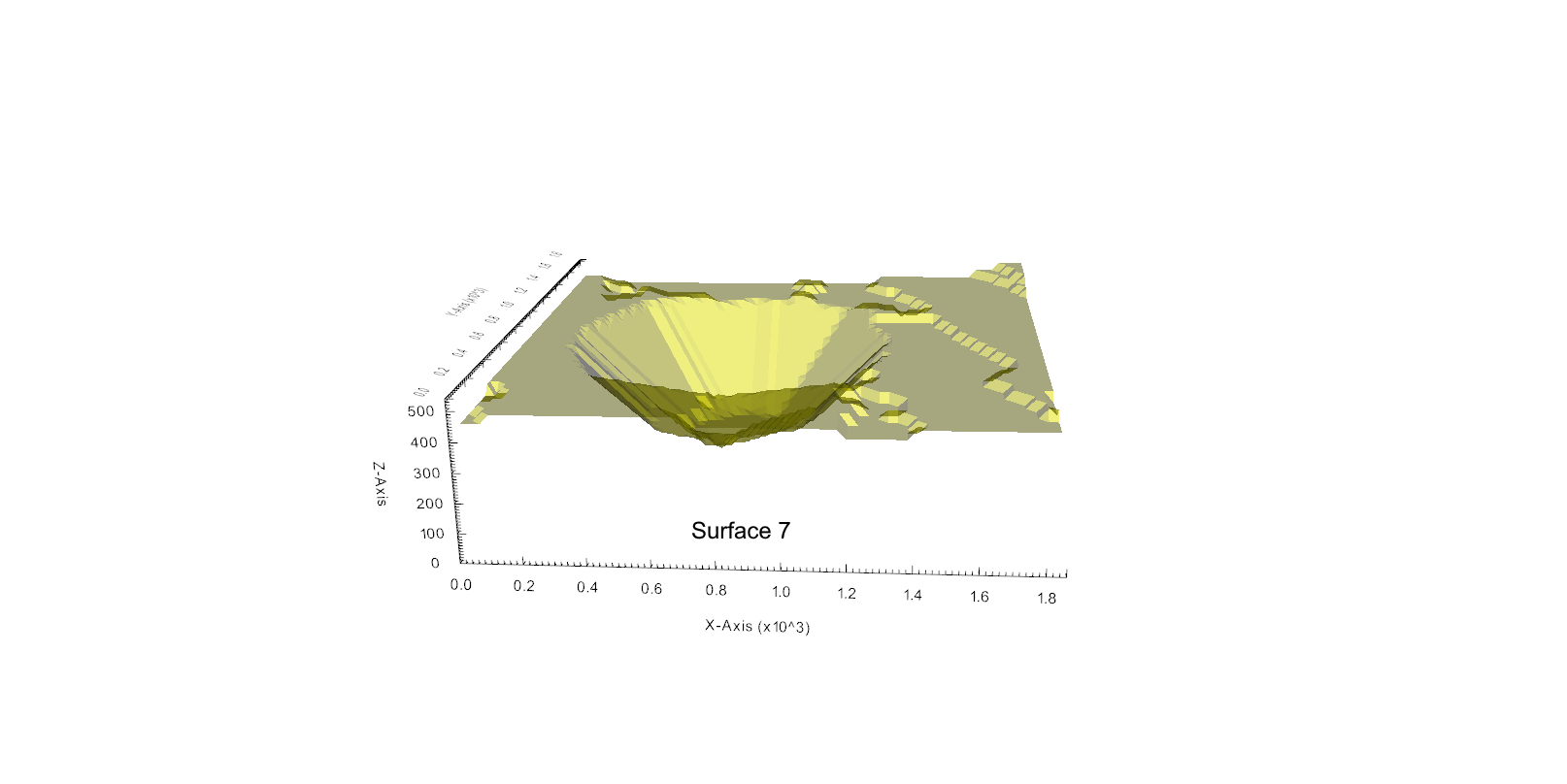
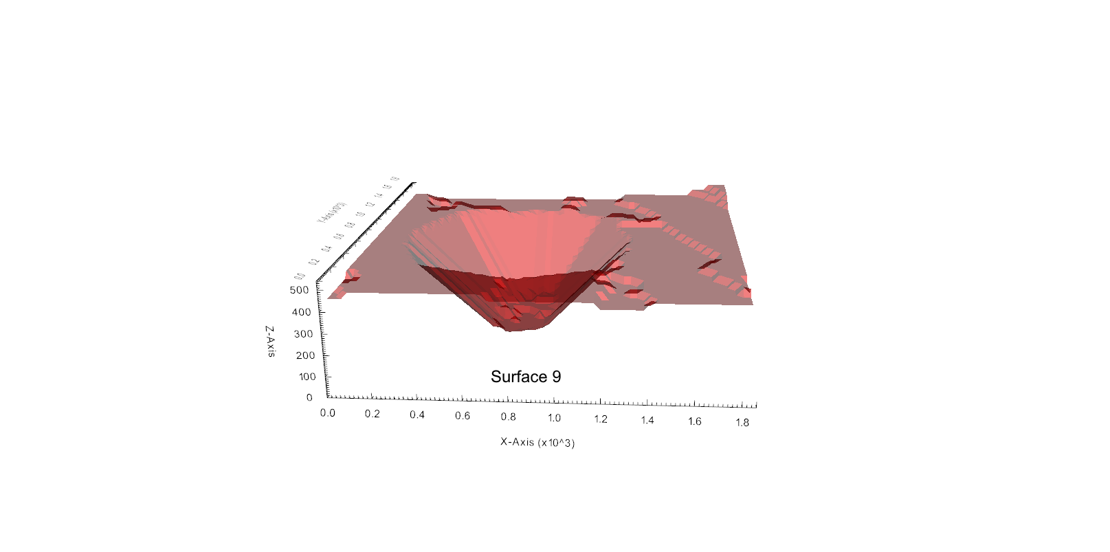
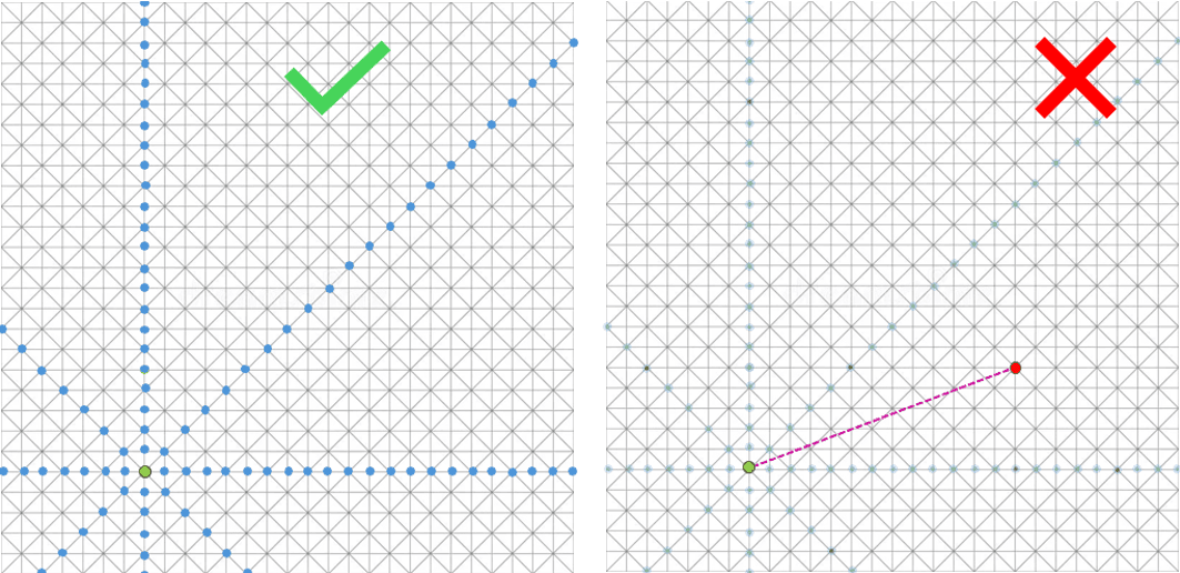
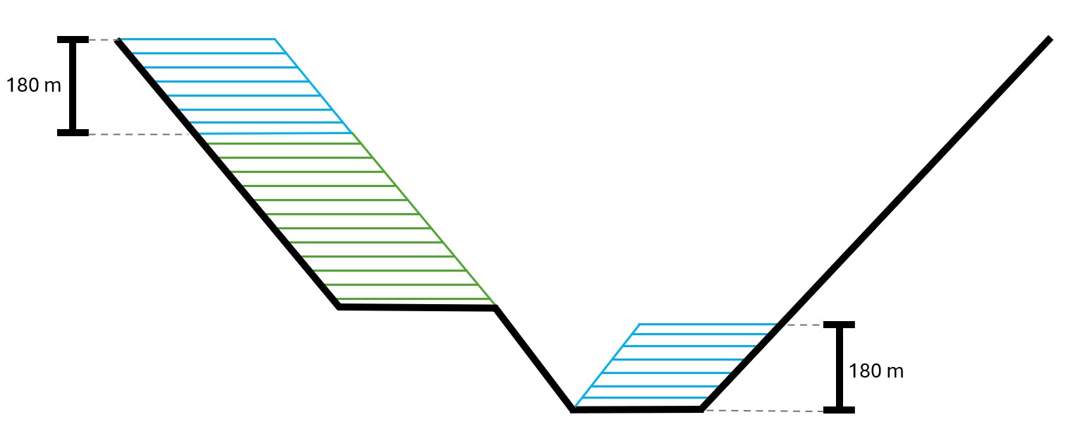
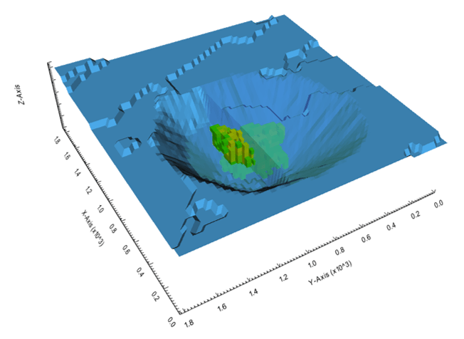
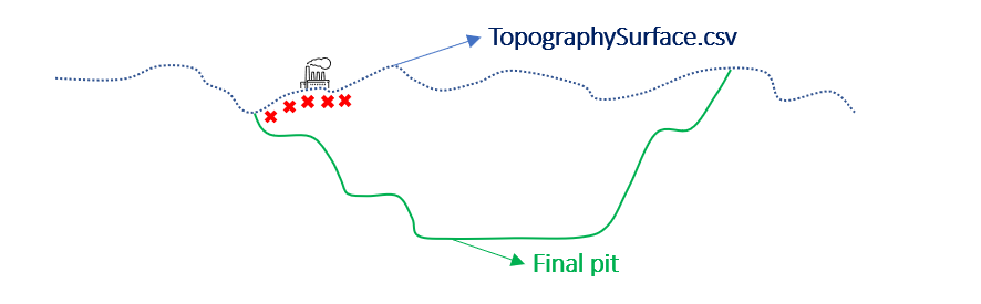
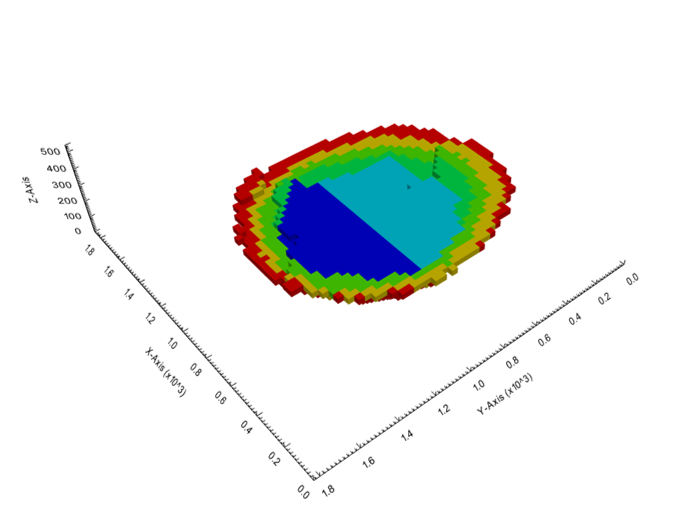
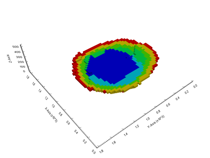
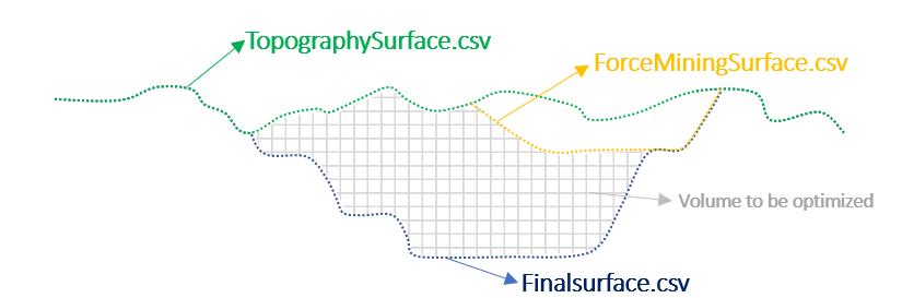
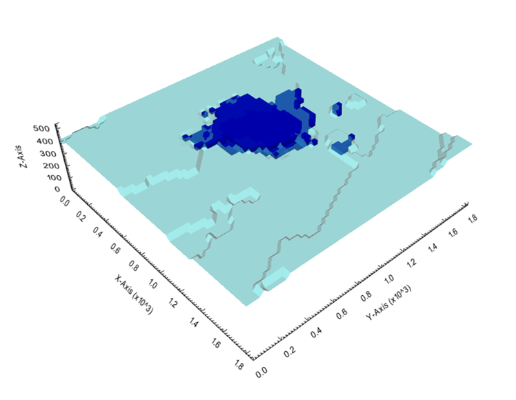
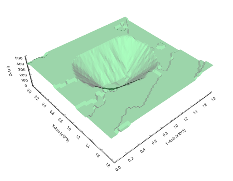
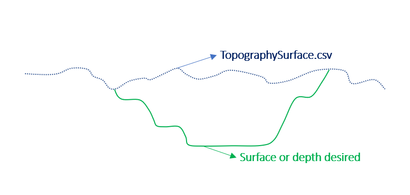
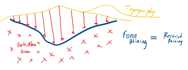
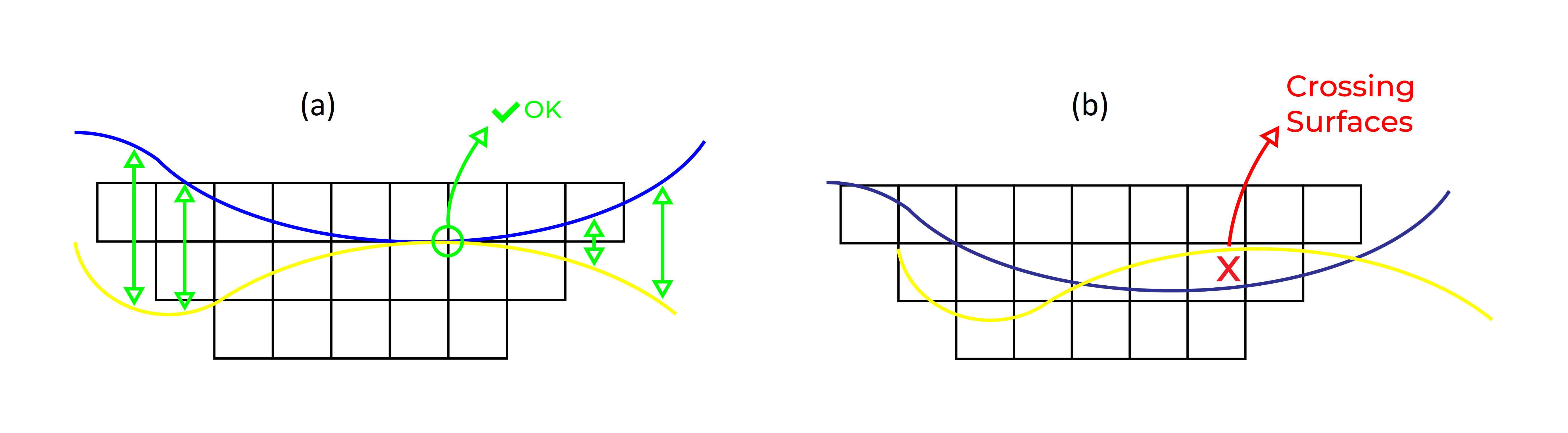 Figure 3: Two surfaces (blue and yellow): a) not crossing each other and respecting the constraint; b) crossing each other and not respecting the constraint.[/caption]
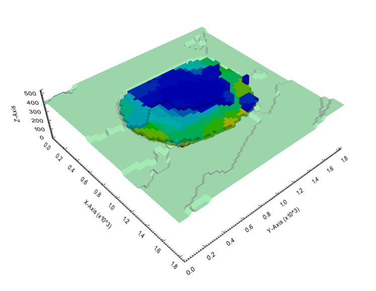
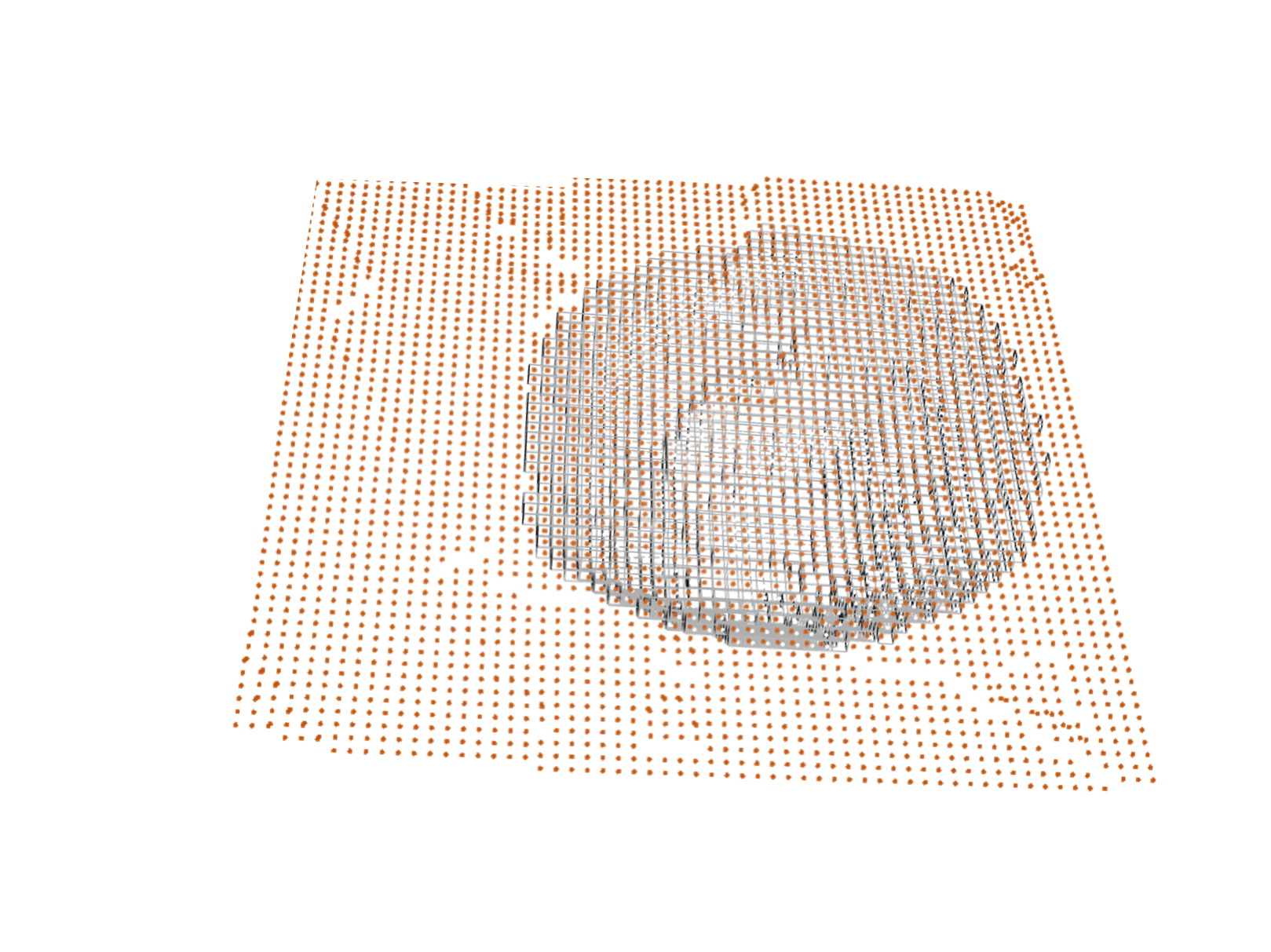
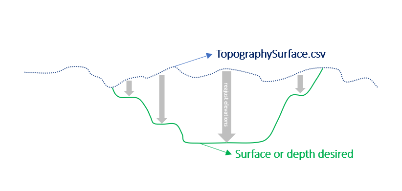
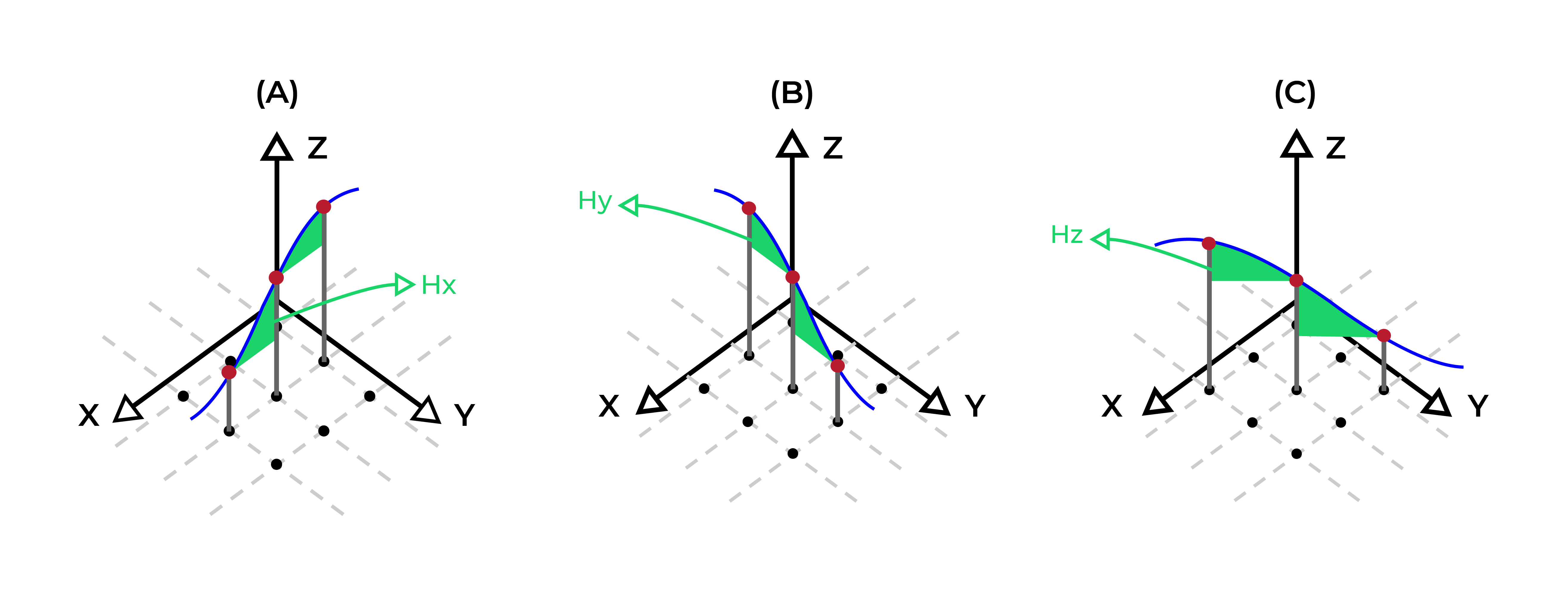 Figure 4: Maximum allowed difference (Hx, Hy, and Hd) in elevation between adjacent cells in contact laterally in the x direction (a), in contact laterally in the y direction (b), and in contact diagonally (c).[/caption]


 “The software that could revolutionize mine planning”
 How digital innovation can improve mining productivity
 A tool for these times
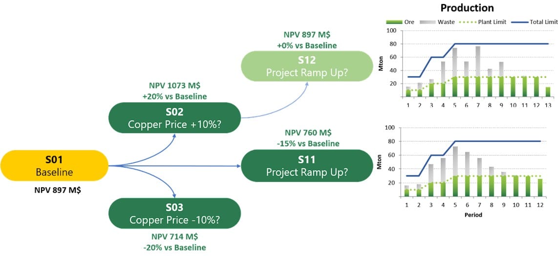
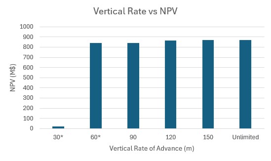
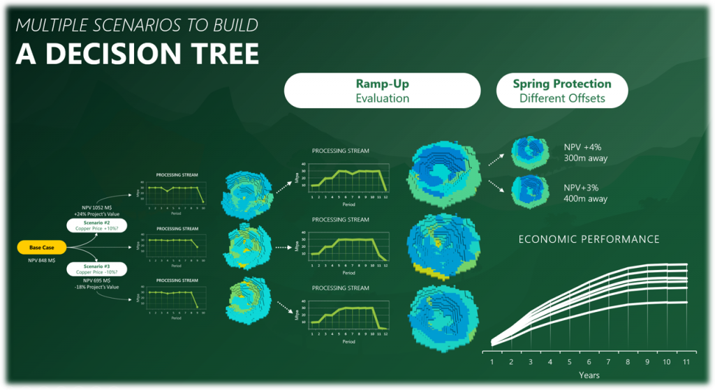
 Mine Optimizations and SimSched DBS is a friend of yours now. SimSched DBS is the most powerful tool to achieve and compare NPV results of the pit.