
Optimized Pushbacks
Highlights
Generating optimized pushbacks is crucial for aligning production volume with economic viability and operational constraints on site.
- Maximizes NPV while respecting physical limits – MiningMath integrates all constraints (geometric, tonnage, blending) in a single run to identify the best pushback volumes that drive higher net present value.
- Fast scenario iteration across timeframes – Its one‑step, simultaneous optimization of multiple period granularities (e.g., 3‑, 5‑, 10‑yr) cuts manual rework and lets teams rapidly compare operational outputs and NPV impacts.
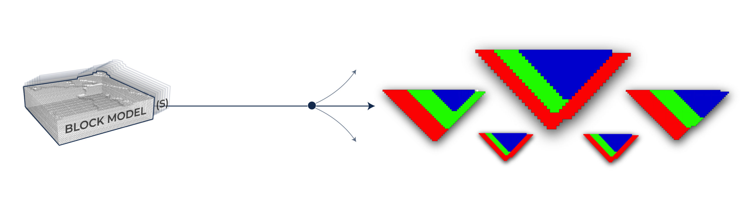
- Operationally realistic designs via block‑model‑direct generation – By producing pushbacks directly from the block model, MiningMath provides mineable shapes that already factor in ramp design and equipment limits, reducing reliance on post‑processing edits.
MiningMath offers the option of producing optimized, single-step pushbacks with controlled ore production and operational designs. This procedure is important to ensure the financial and operational viability of the mining project, as excessively large volumes can render the project unfeasible, while excessively small volumes can result in resource wastage or missed opportunities for ore extraction.
By testing different volumes, it is possible to find an optimal point that maximizes the net present value (NPV) of the project.
How does it work?
MiningMath utilizes timeframes to generate pushbacks at different levels of detail. Timeframes are time intervals that divide the mine’s lifespan into smaller periods. Different timeframes allow users to perform a fast evaluation of the impact of production volume on the NPV. If necessary, adjustments can be made to optimize production and reduce costs.
In Pushback Optimization, multiple optimized pushback scenarios are created with varying levels of detail, enabling users to have a comprehensive view of the impact of volume variations on the project’s performance.
Single-step approach
Every pushback produced with MiningMath is created in a single-step, straight from block model, taking into consideration geometric constraints such as minimum bottom width and minimum mining width, controlling tonnages, blending and other requirements.
Multiple single-step pushback scenarios can be created with varying levels of detail, enabling users to have a a higher variety of options and a comprehensive view of the impact of volume variations on the project’s performance.
Create a Pushback
You can Identify timeframe intervals in your project, so that you can work with group periods before getting into a detailed insight. This strategy allows you to run the scenarios faster without losing flexibility or adding dilution for the optimization, which happens when we reblock.
The idea is to make each optimized period represent biennial, triennial, or decennial plans. MiningMath allows you to do it easily by simply adjusting some constraints to fit with the timeframe selected. Notice that in this example, the processing was not fully achieved, and this kind of approach helps us to understand which constraints are interfering the most in the results.
Tips!
Try to run with and without dump/total productions to check potential bottlenecks and impacts on waste profiles, which could be useful for fleet management exercises. Also, test with wider mining widths than required, as this is a complex non-linear constraint and you might find better shapes without losing value.
Example
Required dataset
Preinstalled Marvin deposit. It can also be downloaded here.
| Property | Value |
|---|---|
Timeframe custom factor | 5 |
Processing capacity | 50Mt in 5 years |
Dump capacty | 150Mt in 5 years |
Vertical rate of advance | 750 m in 5 years |
Minimum Mining Width | 100m |
Minimum Bottom Width | 100m |
Restrict Mining Surface | Optional |
Grade copper | 0.88% |
Stockpiling parameters | On |
Note: Waste control and vertical rate of advance are not recommended if you are just looking for pushback shapes.
Work Through Different Timeframes
Given the previous initial scenario, you might want to consider different timeframes for your pushback design. In order to perform a Pushback Optimization, the timeframes (in green), process and dump production limits (in green) and the vertical rate (in red) will be adjusted.
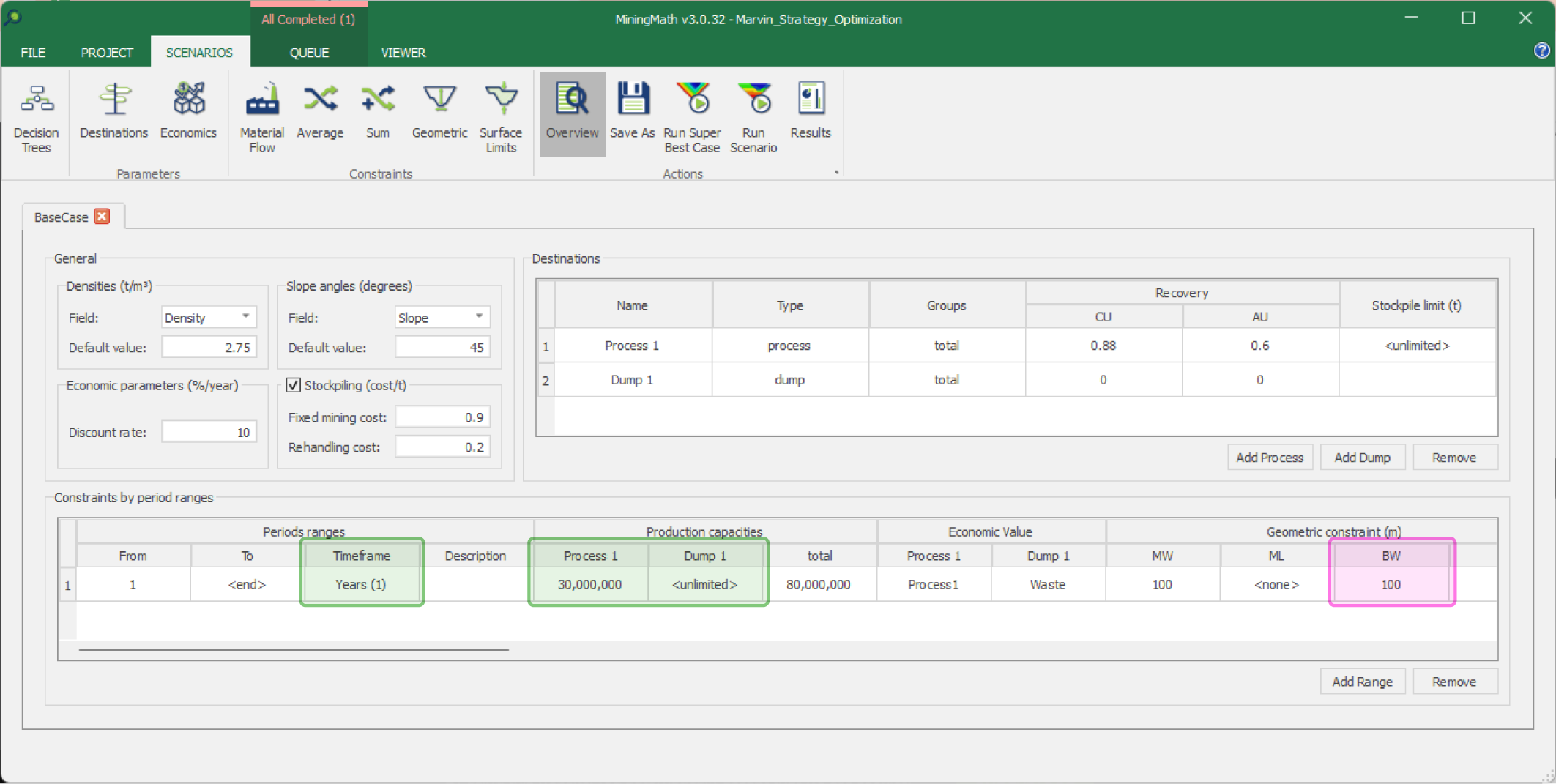
By varying the highlighted parameters above, the following decision tree has been constructed for Pushback Optimization.
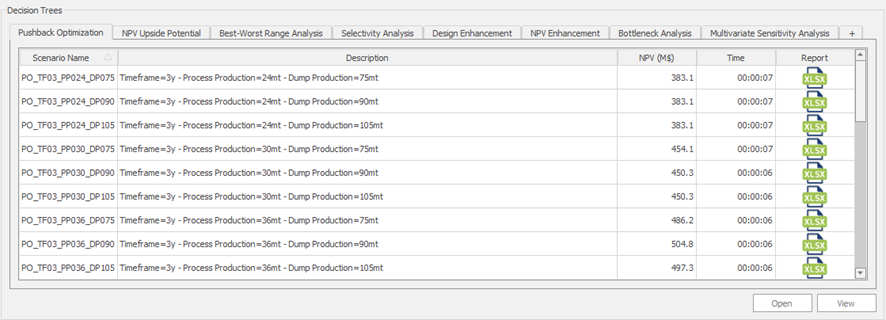
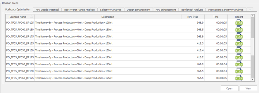
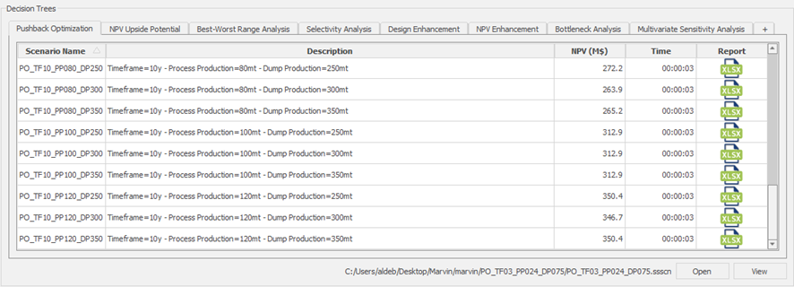
Three different timeframes are explored: 3 years, 5 years, and 10 years. Each timeframe is associated with specific process and dump production limits. Such limits not only scale with their respective timeframes but also allow for variations that provide flexibility for testing different production scenarios. Finally, the vertical rate is also adjusted to align with the defined timeframe of each scenario. For instance, the vertical rate is set to 450m for the 3-year timeframe, 750m for the 5-year timeframe, and 1500m for the 10-year timeframe.
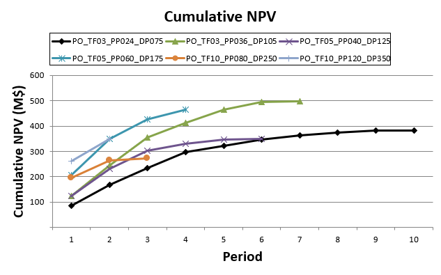
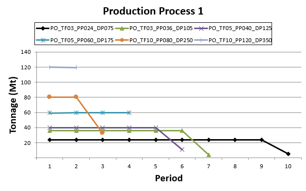
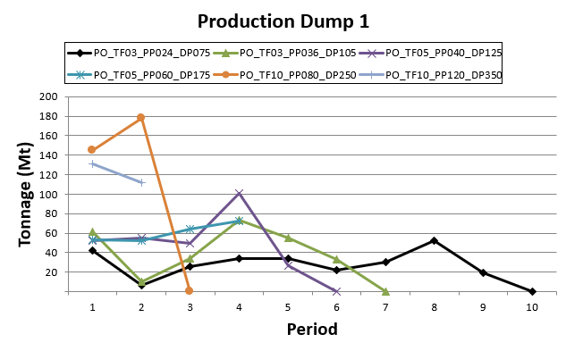
Afterward, specific results were carefully selected for comparison, focusing on key parameters such as Net Present Value (NPV), production process, and production dump.
More details
The 2 constraints inputted at the production tab are related to the maximum material handling allowed: the third one is about the processing equipment capacity, and the vertical rate of advance is related to the depth that could be achieved adjusted to this interval. The minimum mining width was added because we are already generating designed surfaces that could be used later as guidance of detailed schedules, thus, it should respect the parameter due to the equipment sizing. Parameters such as average, minimum bottom and restrict mining surface, don’t suffer any change in the time frames.
It’s important to remember that the packages of time here don’t necessarily have to correspond to identical sets of years. You could propose intervals with different constraints until reaching reasonable/achievable shapes for the design of ramps, for example. If you wish to produce more operational results, easier to design, and closer to real-life operations, try to play with wider mining/bottom widths rates. Those changes will not necessarily reduce the NPV of your project.
Considering this approach the discount rate serves just a rough NPV approximation and it doesn’t affect much the quality of the solution, given that the best materials following the required constraints will be allocated to the first packages anyway.