Selectivity Analysis

Estimated reading: 3 minutes 204 views

Selectivity Analysis is the process of generating and analyzing scenarios to measure the impact of all geometric constraints on the project’s net present value (NPV), from the most selective to the least selective setup. Analyzing the impact of variations in geometric constraints is important to determine the optimal mine configuration and optimize productivity and profit.

By performing such an analysis, it is possible to identify the effect of geometric limitations on mining operations. Moreover, it is possible to evaluate the influence of each parameter and its variation on mine performance. This allows finding the best combination of parameters and mining techniques aimed at maximizing production and profit for each scenario.

In a Selectivity Analysis, scenarios are created including each geometric constraint sequentially and gradually increasing or decreasing their values from the least selective until the desirable requirement. This allows users to have a comprehensive view of the impact of geometric limitations on the project’s performance.

Considering the nature of global optimization and the non-linearity of the problem, it is expected that there will be variations in performance (NPV, production, amount of mine fronts, etc.) as parameter values are modified. Therefore, it is crucial to generate a large number of scenarios to perform a comprehensive analysis of the impact of these variations on the project.

Example

Dataset: Preinstalled Marvin deposit. It can also be downloaded here.

Consider the following base scenario and decision tree built for a Selectivity Analysis using the Marvin dataset.

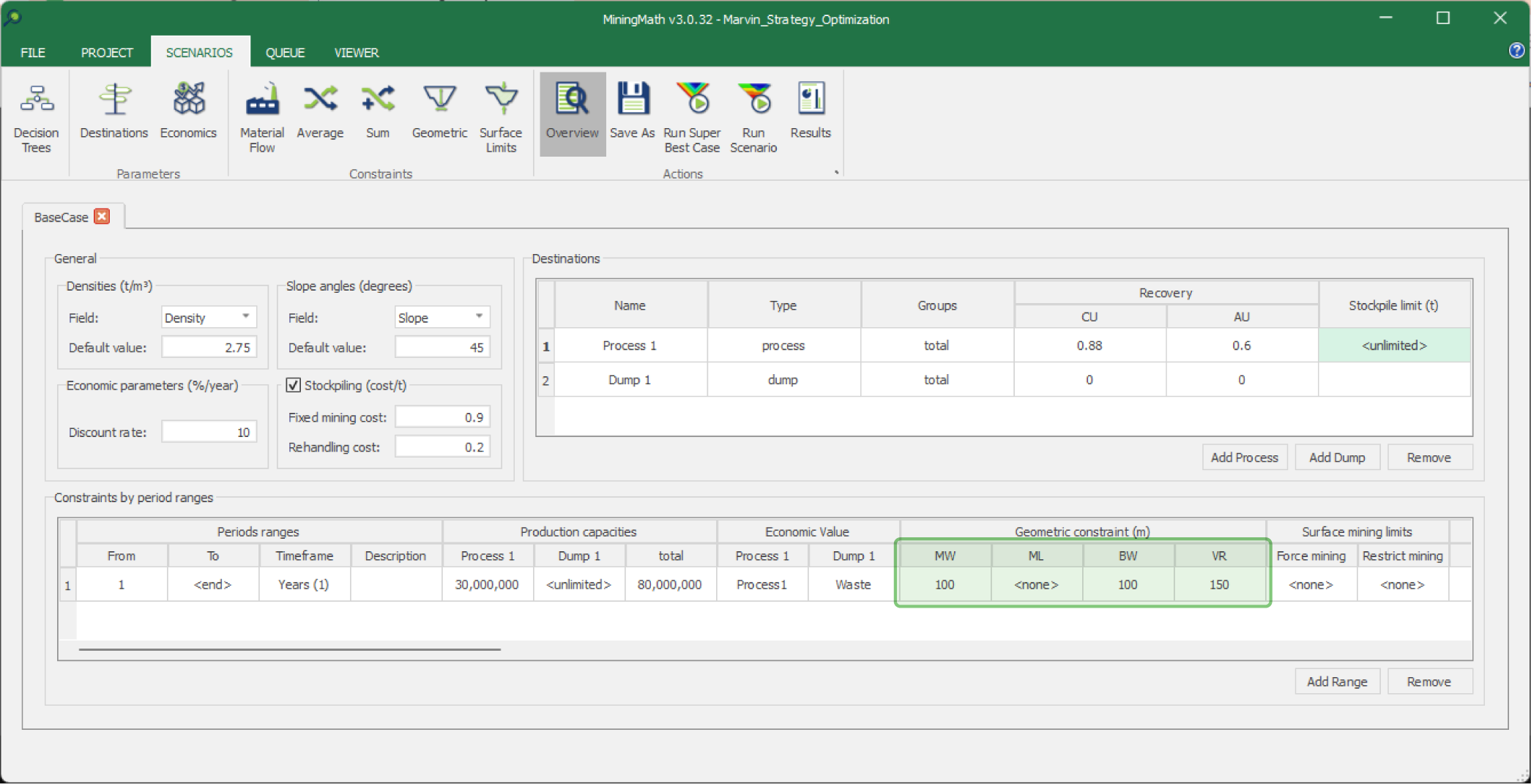
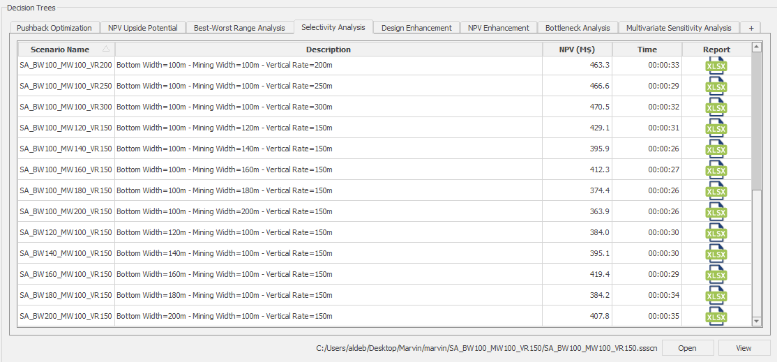
The goal is to understand the impact of different values of geometric constraints (mining width, bottom width, and vertical rate of advance). The geometric parameters (in green) will be tested with a range of different values: bottom width with values from 0m up to 200m; mining width with values from 0m up to 200m; and vertical rate of advance with values from 50m up to 300m. In this example, 26 different scenarios were evaluated.

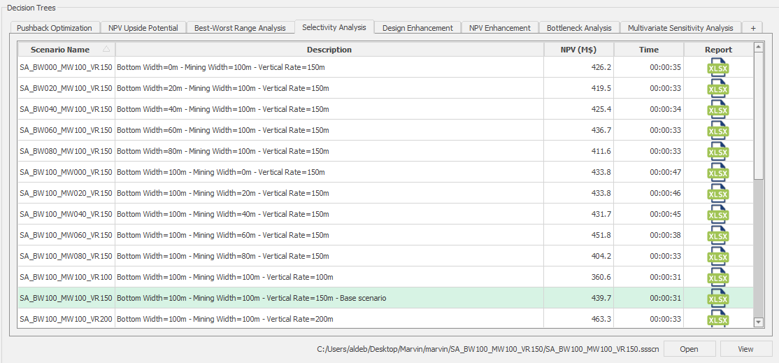
Note that there is no linear relationship between geometric constraints and NPV. In other words, a higher width or lower vertical rate of advance do not necessarily imply a lower NPV. As previously mentioned, that is due to the non-linearity of the problem. The cumulative NPV of the scenarios is compared in the graph below.

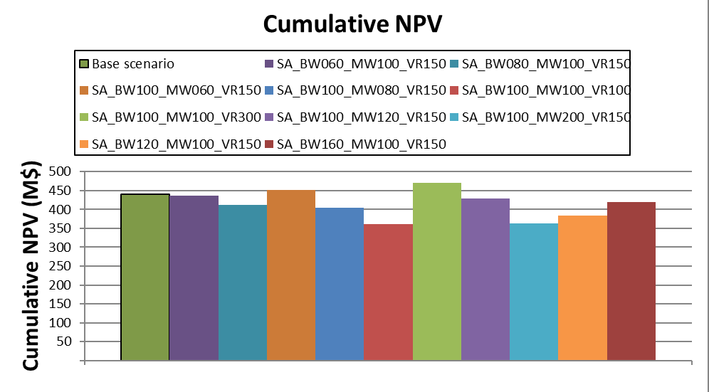
A diverse range of results can be achieved with a Selectivity Analysis. However, there are usually two possibilities when they are compared:

Contrasting geometrics parameters with small NPV variations: note that when the bottom width changes from 0m to 80m, and the remaining parameters are fixed, the NPV drops from 454 M$ to 444M$. This indicates that large changes in geometric constraints do not necessarily lead to large changes in the NPV. The same for the scenarios SA_BW000_MW100_VR150 and SA_BW100_MW100_VR250.
Similar geometric parameters with larger NPV variations: when comparing scenarios SA_BW080_MW100_VR150 and SA_BW100_MW160_VR150 there is a drop in NPV from 444M$ to 370M$, highlighting that the 20m and 60m change in bottom width and mining width respectively can lead to a larger NPV difference in the project.

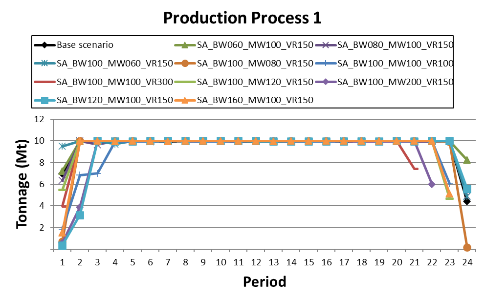
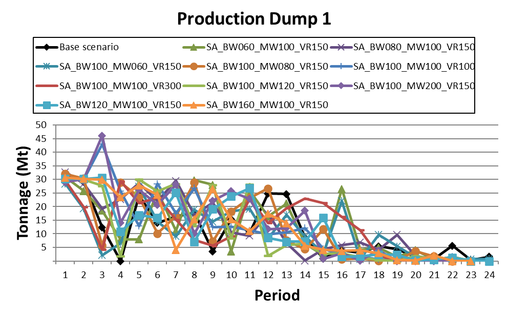
In conclusion, it is important to create several scenarios in a Selectivity Analysis. As exemplified above, results can be quite similar or quite different due to the non-linearity of the problem. Considering the nature of global optimization employed in MiningMath, it is also important to evaluate other indicators. The figures below depict the tonnage achieved for the production, demonstrating the possible impacts for different geometric constraints.

Tagged:
MM-Full

MiningMath

Loading...

Selectivity Analysis

Example

CONTENTS

MiningMath

Loading...

Selectivity Analysis

Example

Related articles

Selectivity Analysis

CONTENTS