
Super Best Case
Highlights
- The “Super Best Case” run generates a fast upper-bound scenario, reducing trial-and-error and supporting informed strategy discussions.
- MiningMath’s single-step engine uniquely handles all constraints at once, making it easier to evaluate complex plans and share results internally.
In the search for the upside potential for the NPV of a given project, this setup explores the whole solution space without any other constraints but processing capacities and discount rate, in a global multi-period optimization fully focused on maximizing the project’s discounted cashflow.
As MiningMath optimizes all periods simultaneously, without the need for revenue factors, it has the potential to find higher NPVs than traditional procedures based on LG/Pseudoflow nested pits, which do not account for processing capacities (gap problems), destination optimization and discount rate. Traditionally, these, and many other, real-life aspects are only accounted for later, through a stepwise process, limiting the potentials of the project.
MiningMath vs Tradional Technologies
MiningMath’s Super Best Case serves as a reference to challenge the best case obtained by other means, including more recent academic/commercial DBS technologies available. See a detailed comparison of these two approaches below.
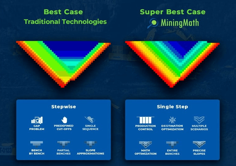
Gap problem and Production Control
In modern/traditional technology, large size differences between consecutive periods may render them impractical, leading to the “gap” problem. Such a gap is caused by a scaling revenue factor that might limit a large area of being mined until some threshold value is tested. MiningMath allows you to control the entire production without oscillations due to our global optimization.
Predefined cut-offs and destination optimization
In the modern/traditional methodology the decisions on block destinations can be taken following some techniques such as: fixed predefined values based on grades/lithologies post-processing cutoff optimization based on economics post-processing based on math programming or even multiple rounds combining these techniques. With MiningMath the destination optimization happens within a global optimization in a single step, maximizing NPV and accounting simultaneously for capacities, sinking rates, widths, discounting, blending, and many other required constraints.
Single Sequence and Multiple Scenarios
Modern technology is restricted to pre-defined, less diverse sequences because it is based on step-wise process built upon revenue factor variation, nested pits, and pushbacks. These steps limit the solution space for the whole process. MiningMath performs a global optimization, without previous steps limiting the solution space at each change. Hence, a completely different scenario can appear, increasing the variety of solutions.
Bench by Bench and Math Optimization
In the modern technology the mining sequence is done following an order of benches inside the pre-defined pits’ order. In MiningMath that is not necessary. The mathematical optimization is done
in a single step through the use of surfaces, not being bound to fixed benches.
Partial Benches and Entire Benches
Due to tonnage restrictions, modern technology might need to mine partial benches in certain periods. With MiningMath’s technology, there isn’t such a division. MiningMath navigates through the solution space by using surfaces that will never result in split benches, leading to a more precise optimization.
Slope Approximations and Precise Slopes
Modern approaches present a difference between the optimization input parameters for OSA (Overall Slope Angle) and what is measured from output pit shells, due to the use of the “block precedence” methodology. MiningMath works with “surface-constrained production scheduling” instead. It defines surfaces that describe the group of blocks that should be mined, or not, considering productions required, and points that could be placed anywhere along the Z-axis. This flexibility allows the elevation to be above, below, or matching a block’s centroid, which ensures that MiningMath’s algorithm can control the OSA precisely, with no errors that could have a strong impact on transition zones.
Finding your Super Best Case
Before setting-up your Super Best Case scenario make sure your project data have been successfully imported and validated.
To run a Super Best Case, after running our Validation Wizard, you only need to add two more mandatory constraints: Processing capacity and Discount Rate.
Note:
Depending on your block model and specificities of your project, additional parameters may need to be specified. For example, if you have multiple destinations these could be added for proper destination optimization.
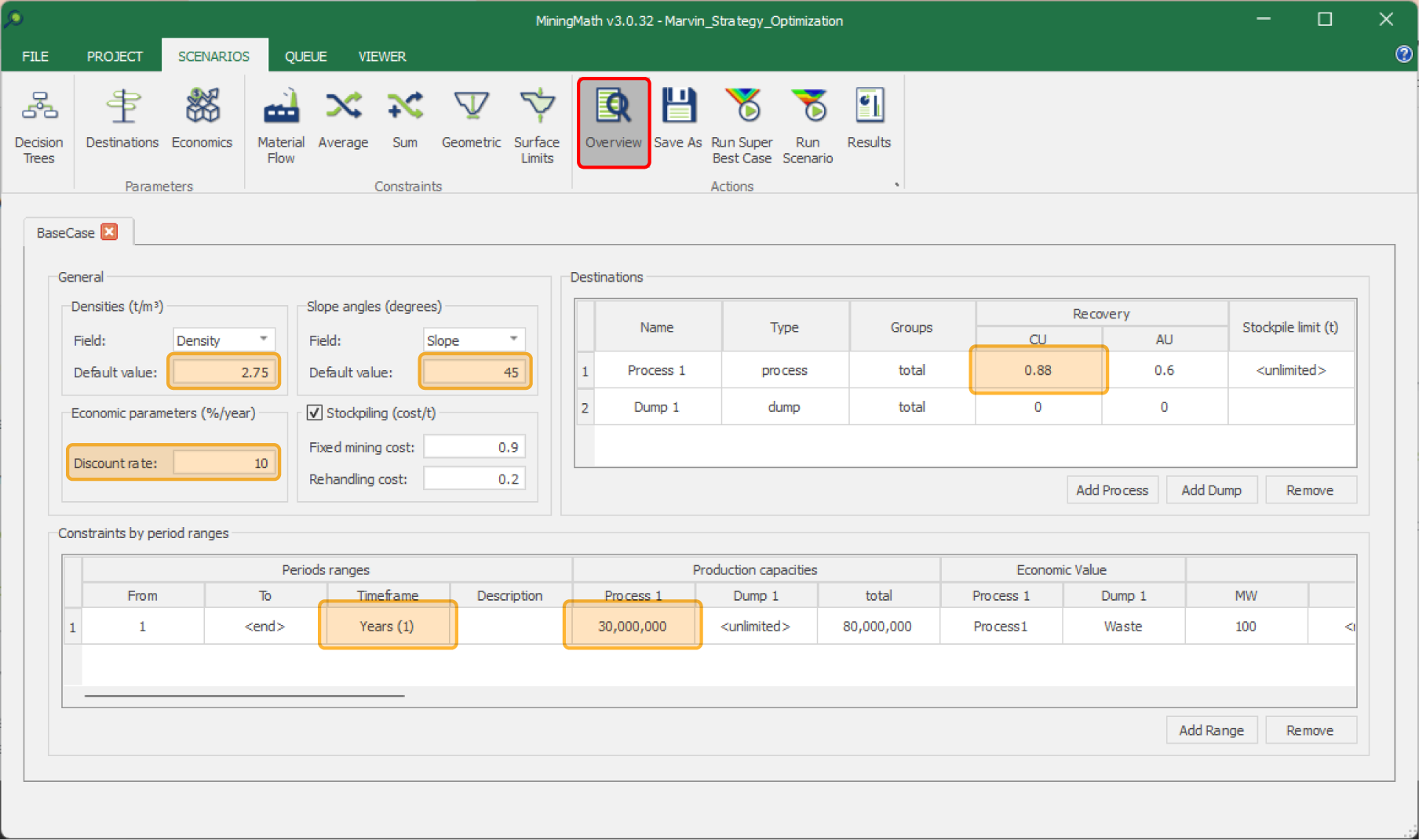
After setting up everything, just hit the “Run” button.
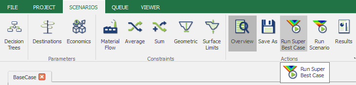
Using the SBC button
If you already have a scenario set up with all your project constraints and want to explore its Super Best Case, there’s no need to change anything.
Simply click the new Run Super Best Case button in your current scenario, and MiningMath will automatically run the analysis, considering only the constraints required for the Super Best Case. This delivers valuable insights into your scenario’s NPV upside potential.
The results are seamlessly integrated into your decision tree and clearly labeled to indicate the original scenario from which the Super Best Case was derived, as shown below:
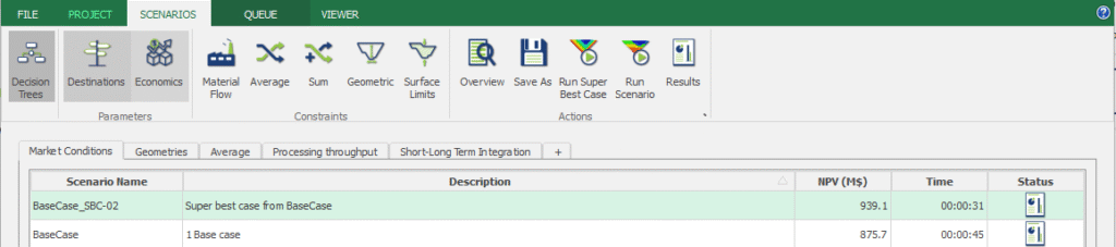
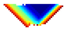
Results
Results can be analysed in the Viewer tab and the exported report file. For the pre-installed Marvin dataset, note how the sequencing has no gap problems, and the production is kept close to the limit without violating any restrictions.


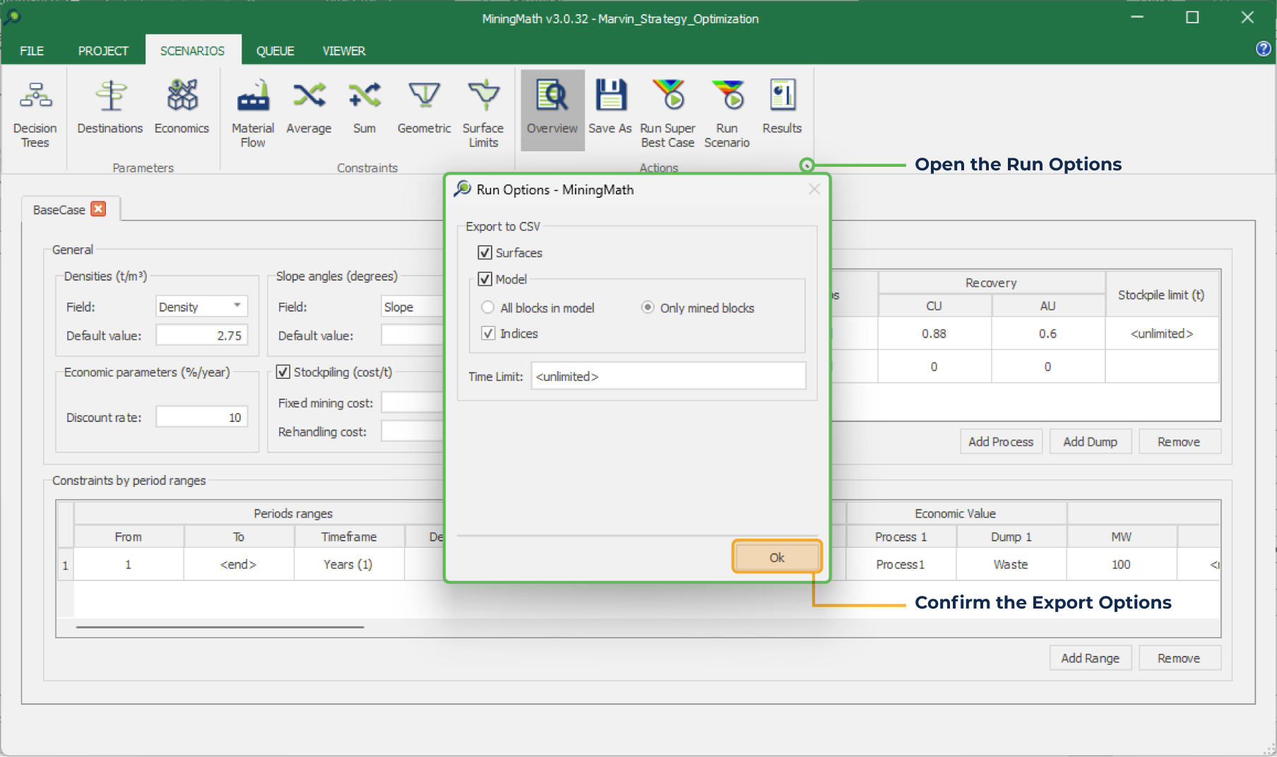
Export files
The block periods and destinations optimized by MiningMath’s Super Best Case (or any other scenario) can be exported in a CSV format. You could use these results to import back into your preferred mining package, for comparison, pushback design or scheduling purposes. Export options are depicted below.
Adding constraints
A refinement of the super best case could be done by adding more constraints, preferably one at the time to evaluate each impact in “reserves”, potential conflicts between them, and so on. You can try to follow the suggestions below for this improvement:
All restrict mining aspects due to forbidden areas.
All force mining aspects for zones that must be mined.
All sum constraints.
All dump and/or total production constraints.
All stockpiles.
Execution time and additional constraints
Adding additional constraints may increase execution time. For running complex scenarios, it’s recommended to use a powerful machine. To facilitate testing and analyzing multiple scenarios, MiningMath now includes a new queuing system (download it here).
