NPV Calculation

MiningMath's internal math for NPV Calculation

The following video explains more about the NPV calculation made by MiningMath’s algorithm. The understand of these steps might be useful for users working on projects with variable mining costs, which are not yet smoothly implemented on the UI.

Video 1: NPV calculation.

Discount rate per period

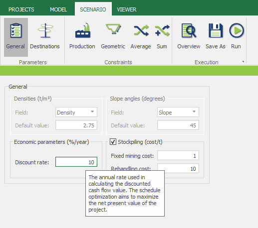
The discount rate (%/year) is provided by the user in MiningMath’s interface, as depicted in the figure below.

Discounted cash flow for annual time frames

In a usual scenario period ranges are defined by annual time frames, as depicted in Fig-2.

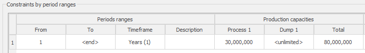
In this case, the annual discount rate multiplier (annual_multiplier) to return the discounted cash flow is performed as follows:

$\text{annual_multiplier}(t) = $ $\frac{1}{(1 + \text{input discount rate})^t}$

The table below exemplifies one case for 10 periods.

Period	Process 1	Dump 1	NPV (Discounted) M$	Annual multiplier	Undiscounted NPV M$
1	P1	Waste	1.2	0.909	1.320
2	P1 +5%	Waste	137.9	0.826	166.859
3	P1 +5%	Waste	132.5	0.751	176.358
4	P1 +5%	Waste	105.4	0.683	154.316
5	P1 -5%	Waste	89	0.621	143.335
6	P1 -5%	Waste	92	0.564	162.984
7	P1 -5%	Waste	91.3	0.513	177.918
8	P1 -10%	Waste	52.3	0.467	112.110
9	P1 -10%	Waste	54.3	0.424	128.037
10	P1 -10%	Waste	12.1	0.386	31.384

Table 1: Example of annual multiplying factors and undiscounted cash-flows for a 10% discount rate per year. Process 1 exemplifies the use of different economic values per period.

In details, Table 1 lists:

the NPV (discounted) resulting from a 10 yearly period with a 10% discount rate per year.
the annual discount rate (annual_multiplier) for each period; and
the undiscounted NPV as the result of the discounted NPV divided by the annual_multiplier.

Discounted cash flow for custom time frames

MiningMath allows the creation of scenarios in which period ranges are defined with custom time frames (months, trienniums, decades, etc.), as depicted in Figure 3.

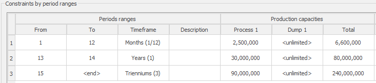
In this case, the discount rate is still provided in years on the interface. However, the discount rate per period follows a different set of calculations. To identity the correct multiplier (discount rate for a custom time frame) applied to each custom time frame, it is necessary to apply the formula below:

$ \text{mult}(t) = \frac{1}{(1 + \text{discount_rate}(t)) ^ {\text{tf_sum}(t)}}$

where:

$
\text{tf_sum}(t) = \sum_{i=1}^{t}\frac{TF(i)}{TF(t)}
$

and

$
\text{discount_rate}(t) = (1 + \text{annual_discount_rate})^{TF(t)} – 1
$

and

$
TF(t)=
\begin{cases}
1,& \text{if}\, t\, \text{is in years}\\
\frac{1}{12},& \text{if}\, t\, \text{is in months}\\ 3,& \text{if}\, t\, \text{is in trienniums}\\
etc.&
\end{cases}
$

For example, to calculate the multiplier of the first period in figure 3, the equation would be:

$ TF(1) = \frac{1}{12} = 0.8333… $

$ \text{tf_sum}(t) = \sum_{i=1}^{1}\frac{TF(1)}{TF(1)} = 1 $

$ \text{discount_rate}(1) = (1 + \text{annual_discount_rate})^{TF(1)} – 1 = (1 + 0.1) ^ {1/12} – 1 = 0.007 $

$ \text{mult}(1) = \frac{1}{(1 + \text{discount_rate}(1)) ^ {\text{tf_sum}(1)}} = \frac{1}{(1 + 0.007)^{1}} = 0.993 $

Another example, to calculate the multiplier of period 15 in figure 3, the equation would be:

$ TF(15) = 3 $

$ \text{tf_sum}(t) = \sum_{i=1}^{15}\frac{TF(i)}{TF(15)} = 2 $

$ \text{discount_rate}(15) = (1 + \text{annual_discount_rate})^{TF(15)} – 1 = (1 + 0.1) ^ {3} – 1 = 0.331 $

$ \text{mult}(15) = \frac{1}{(1 + \text{discount_rate}(15)) ^ {\text{tf_sum}(15)}} = \frac{1}{(1 + 0.331)^{2}} = 0.564 $

MiningMath

Loading...

MiningMath's internal math for NPV Calculation

Discount rate per period

Discounted cash flow for annual time frames

Discounted cash flow for custom time frames

CONTENTS