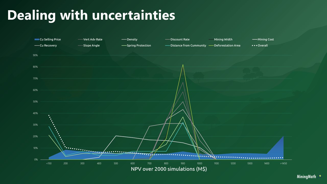
Unexpected Results
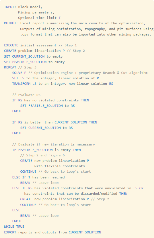
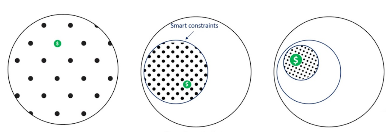
"I’m running MiningMath, but it’s mining a less profitable area, or even waste, or it’s not achieving the specific constraint I’ve set... Why is that?" To understand this, it’s important to recognize that not everything that is aimed to be incorporate into a mining project is mathematically feasible when attempting to respect all constraints simultaneously. Handling multiple,..."
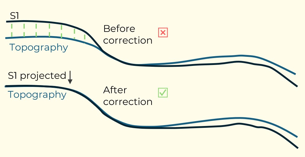
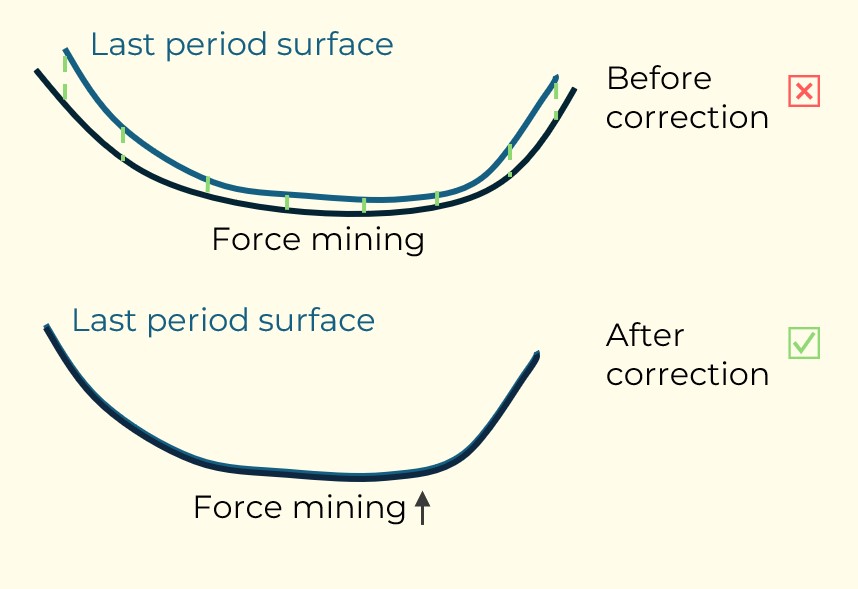
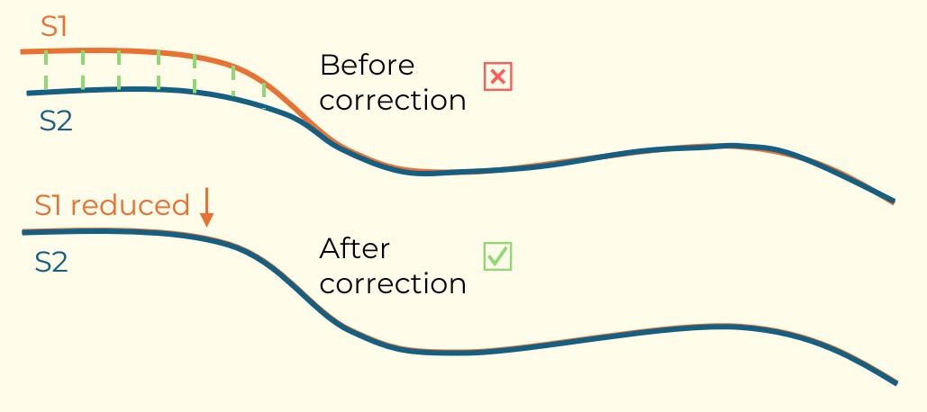
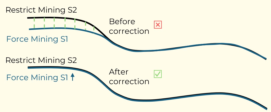
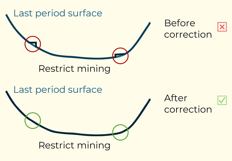
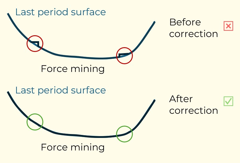
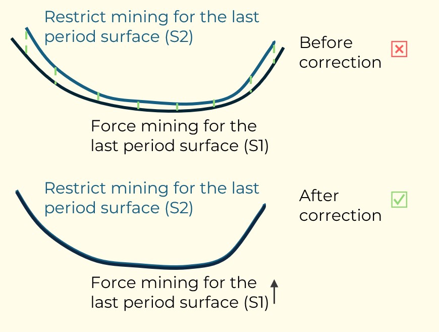
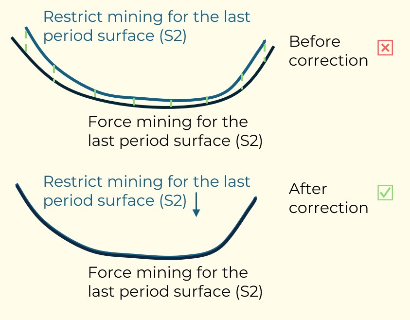
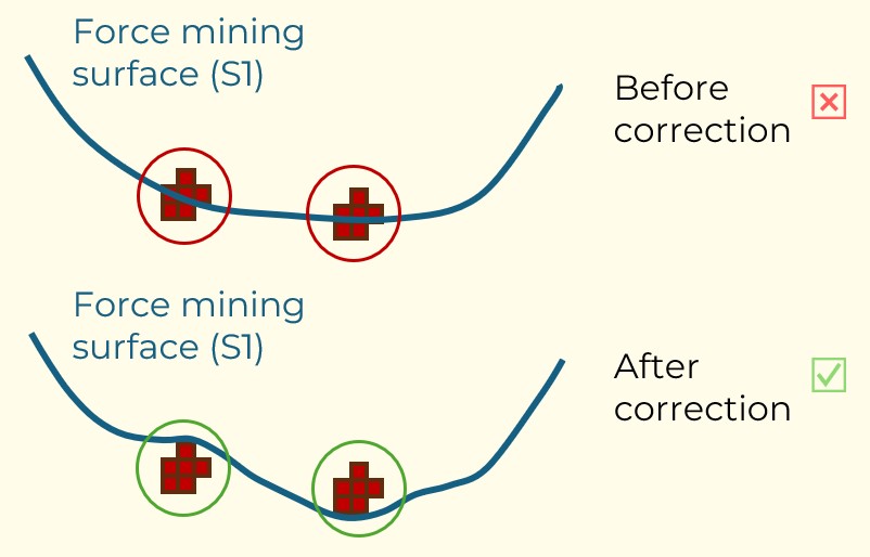
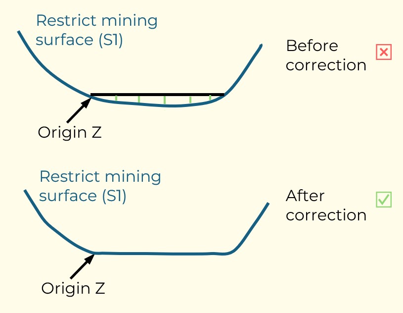
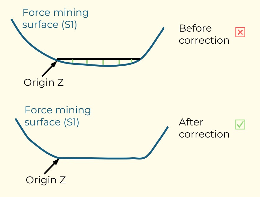
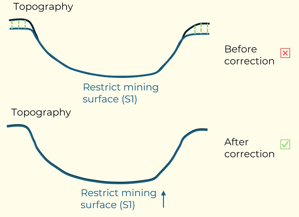
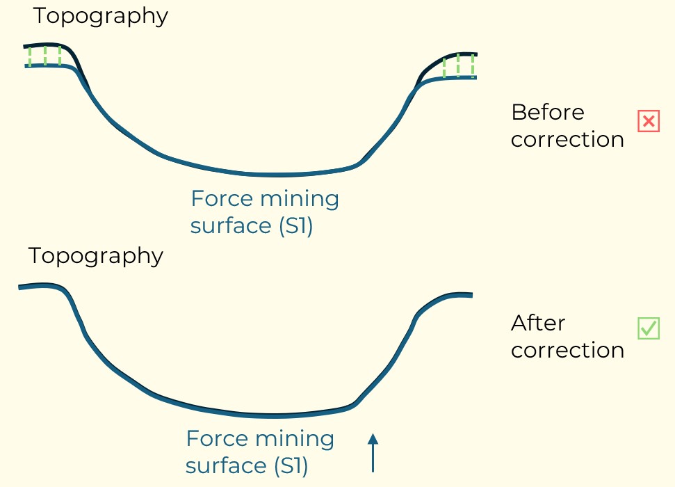
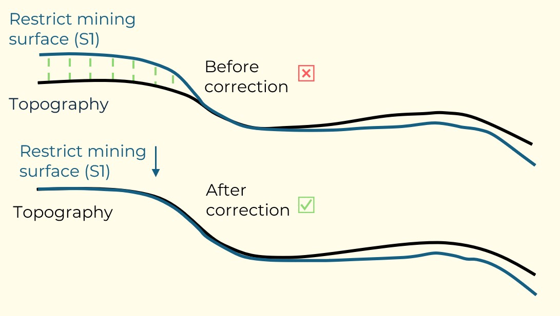
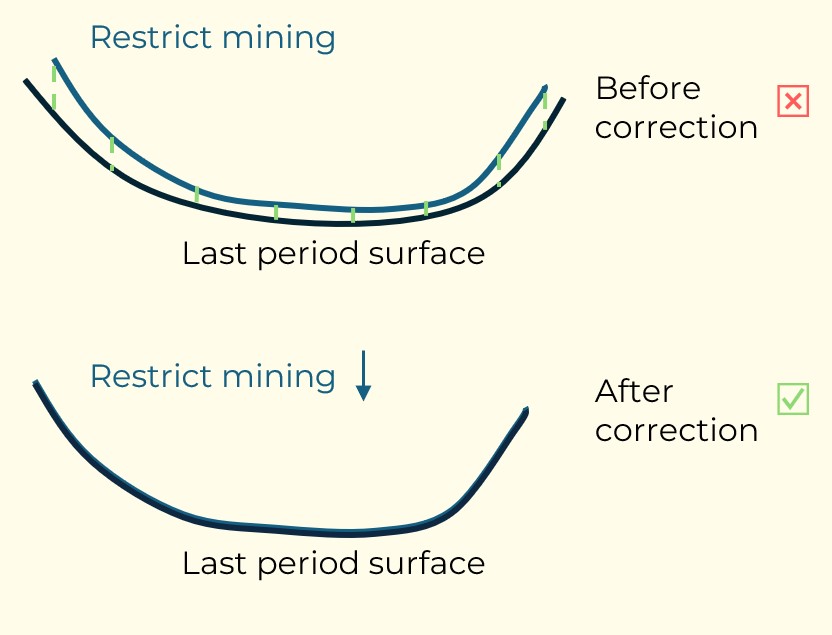
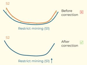
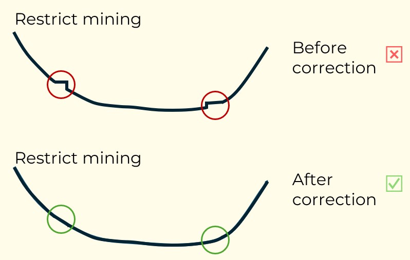
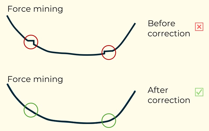

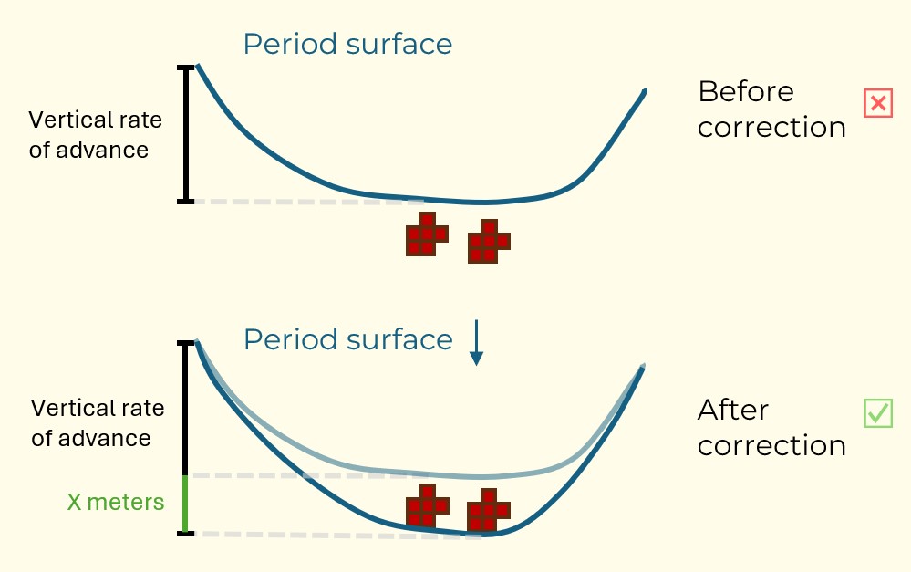


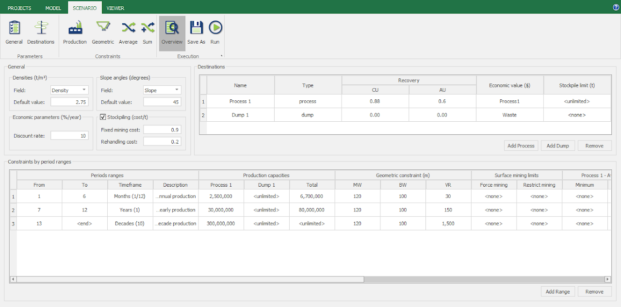

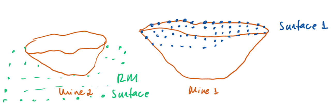
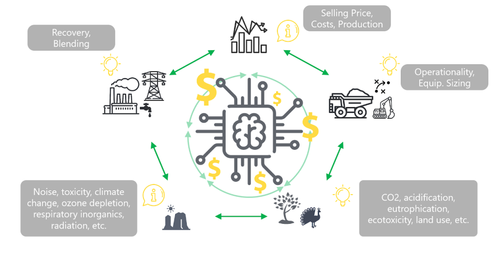
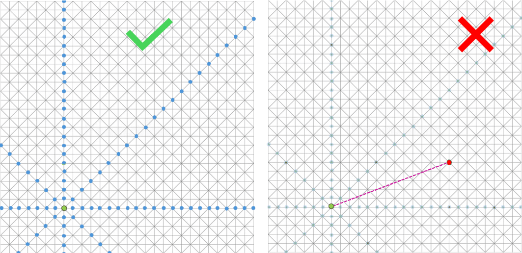
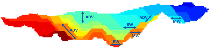
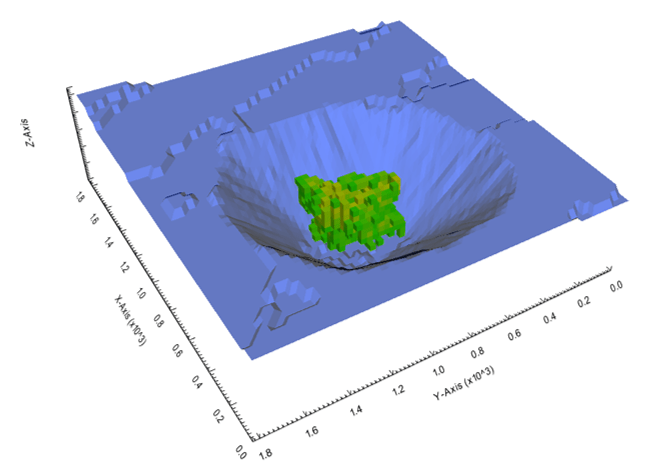
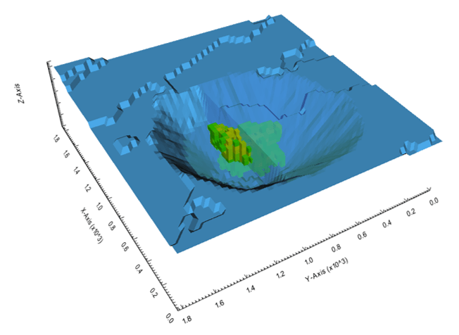
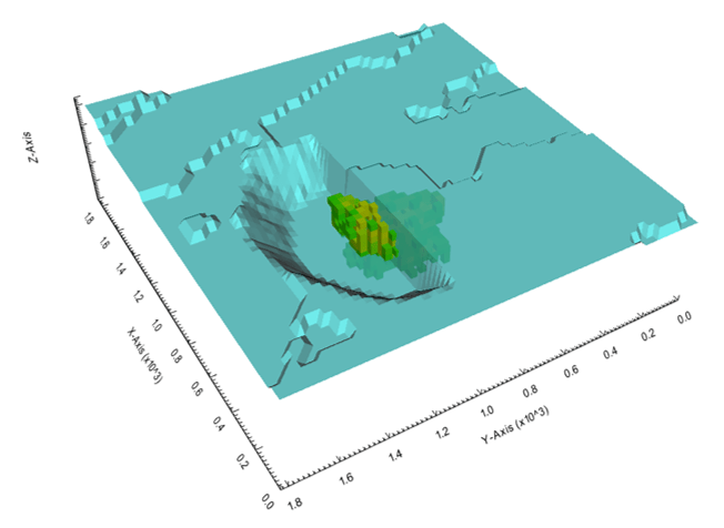
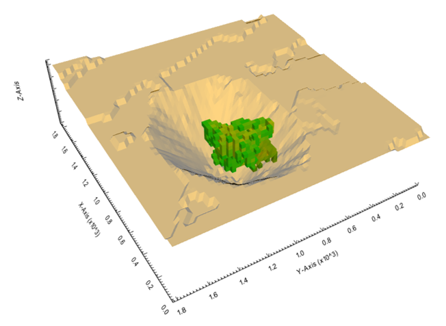
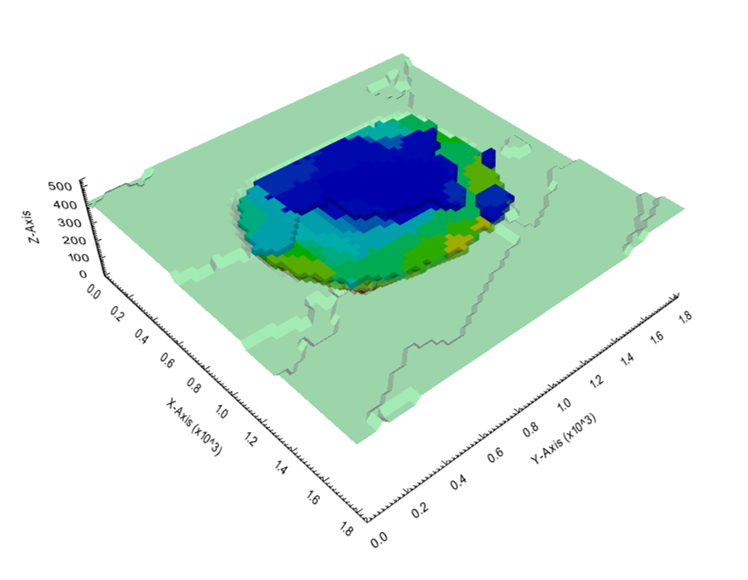
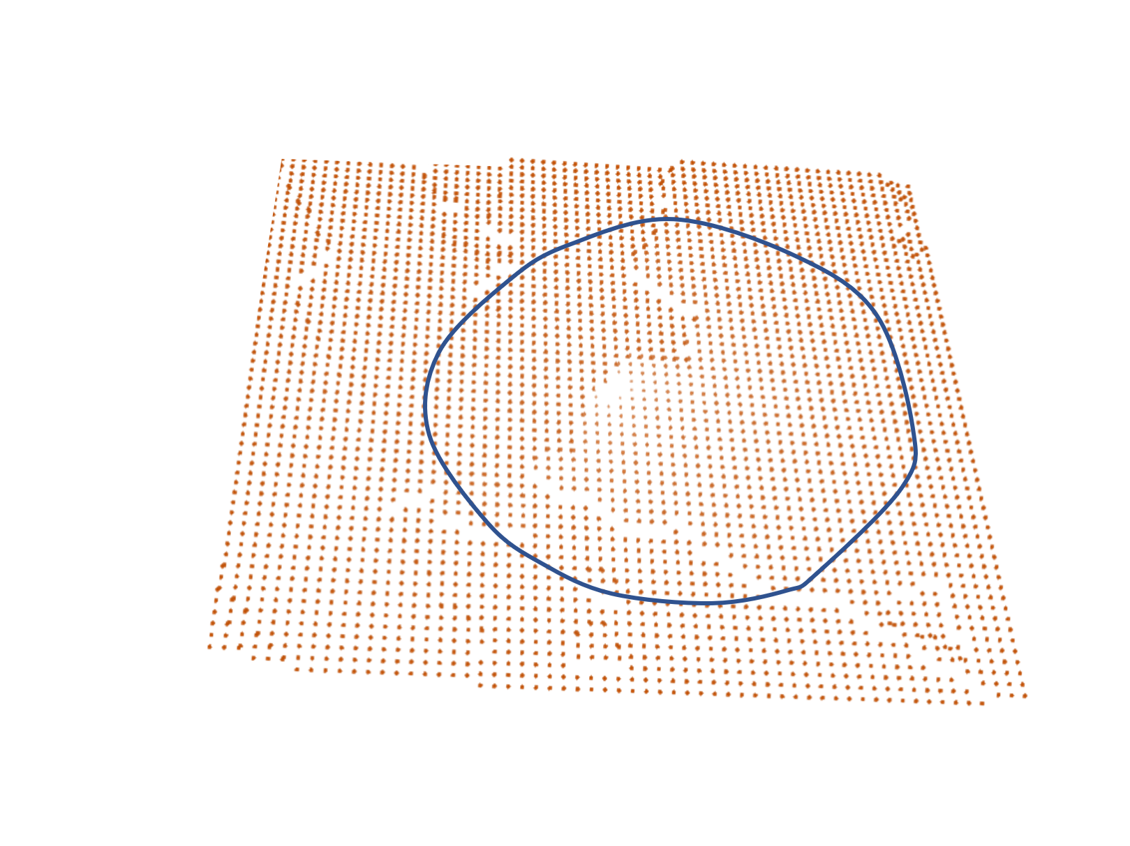
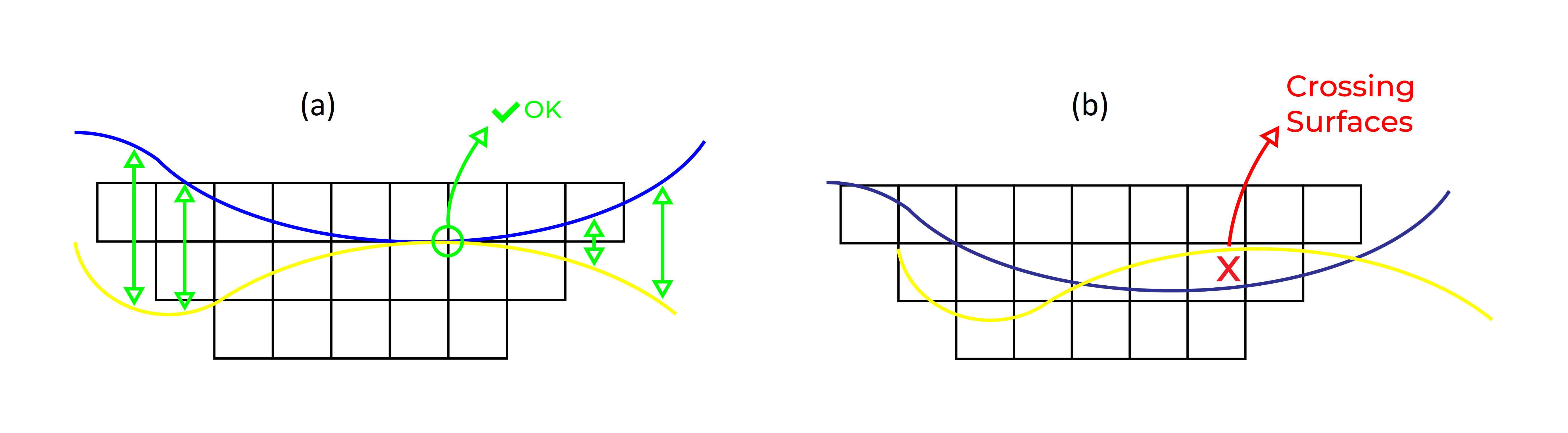 Figure 3: Two surfaces (blue and yellow): a) not crossing each other and respecting the constraint; b) crossing each other and not respecting the constraint.[/caption]
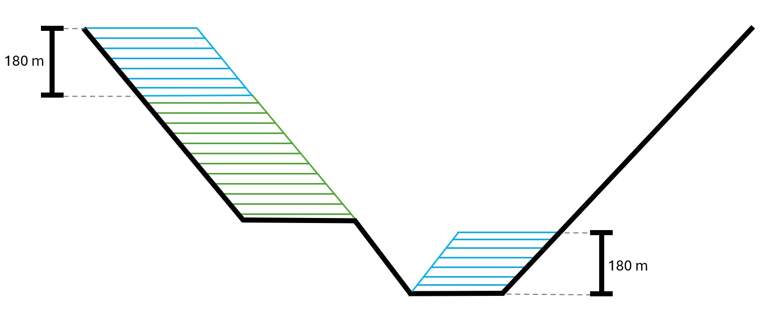
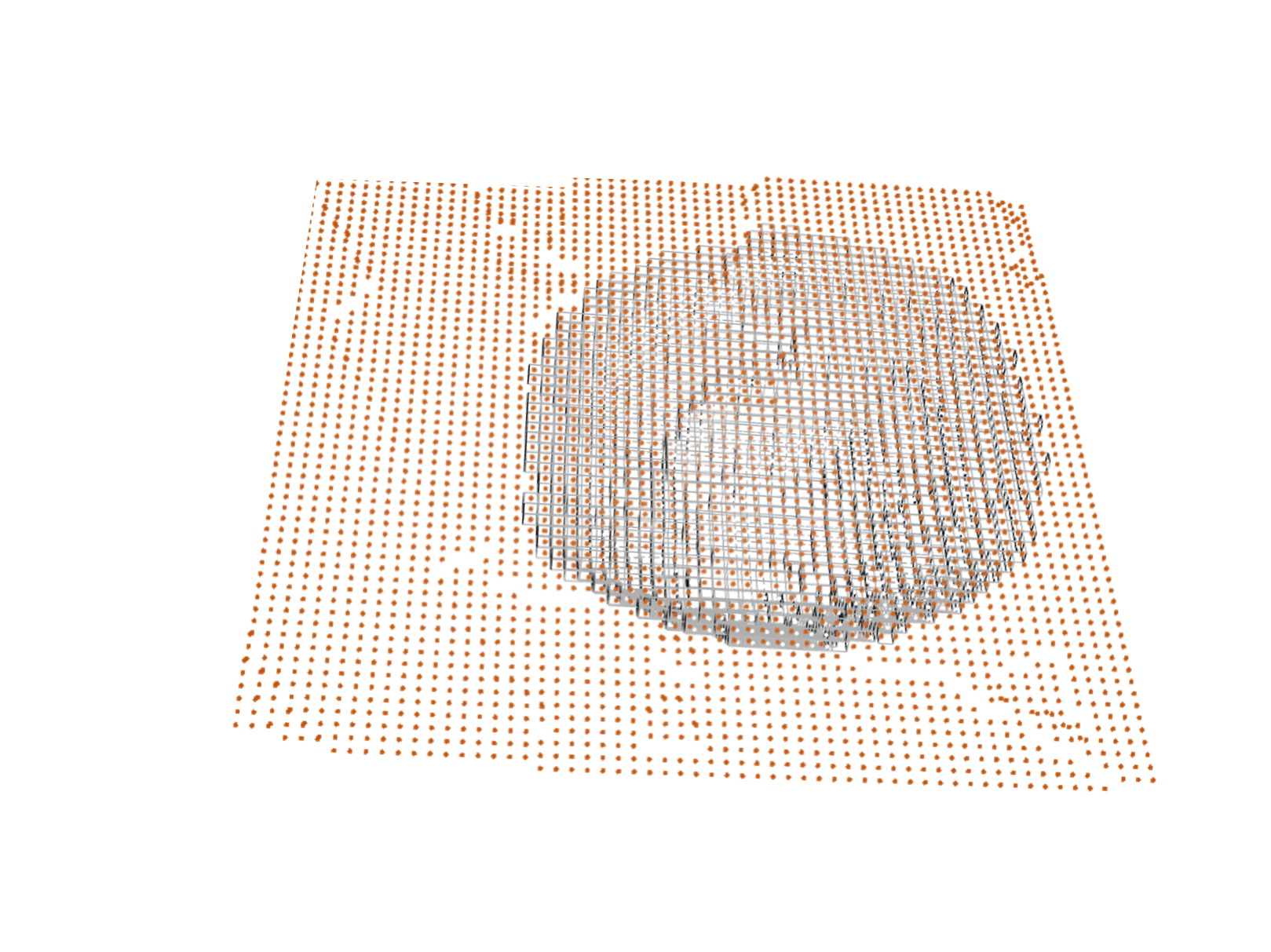
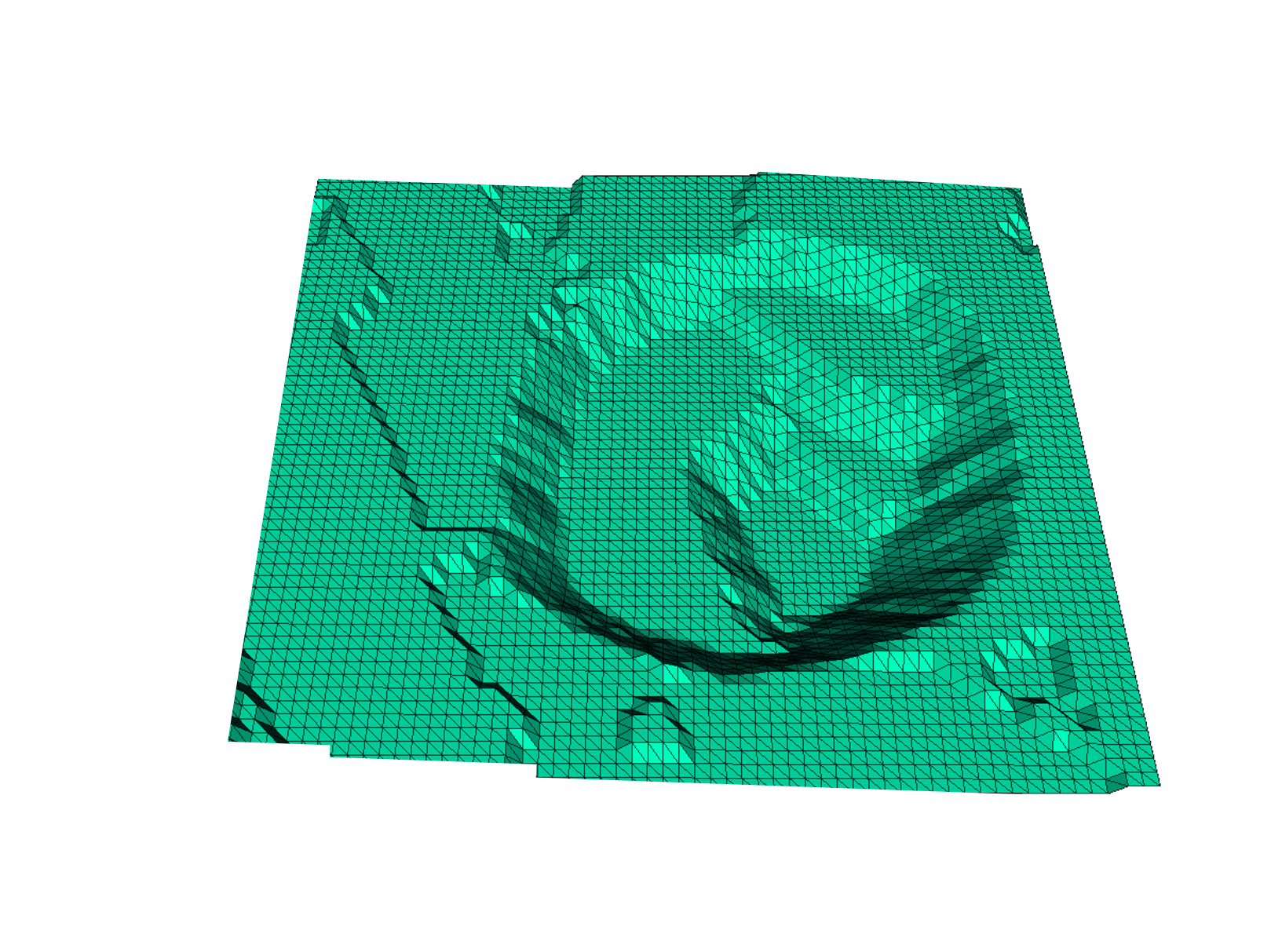
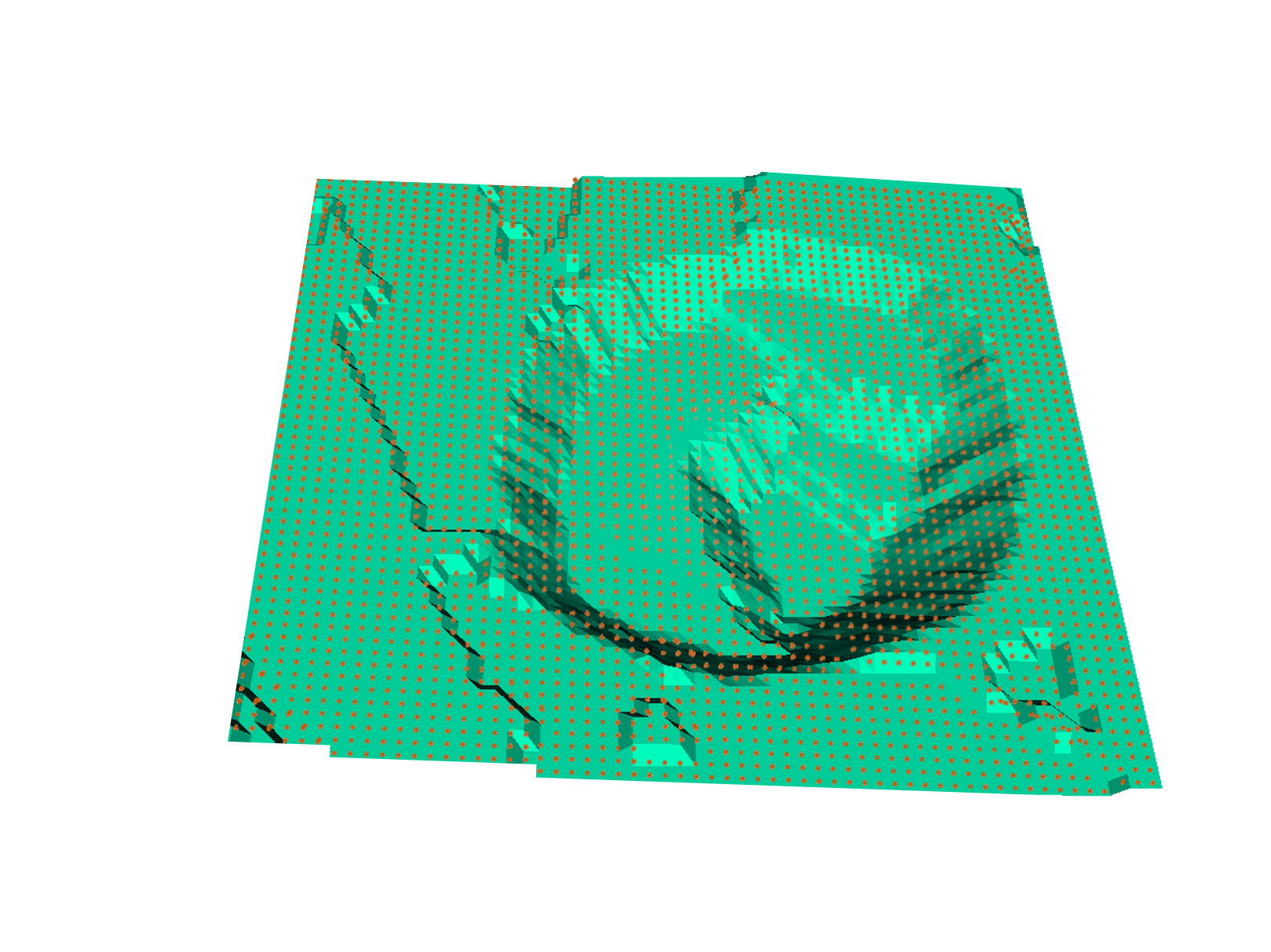
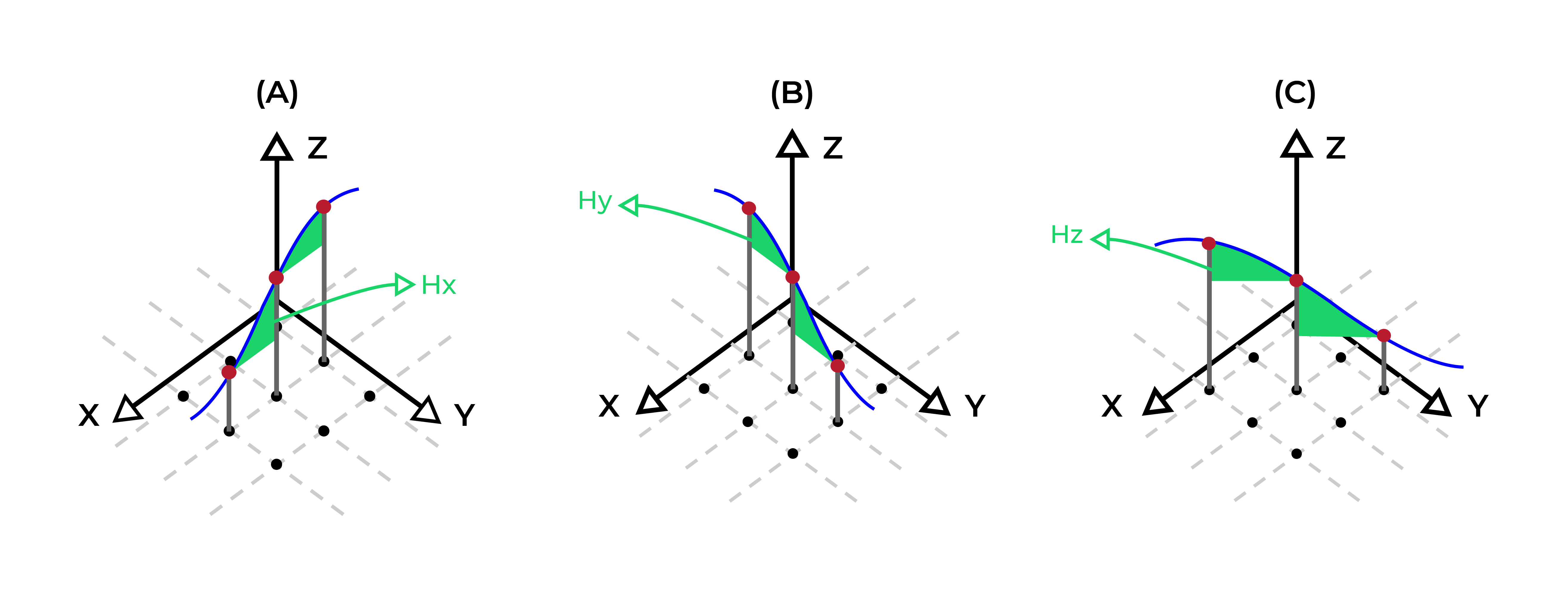 Figure 4: Maximum allowed difference (Hx, Hy, and Hd) in elevation between adjacent cells in contact laterally in the x direction (a), in contact laterally in the y direction (b), and in contact diagonally (c).[/caption]
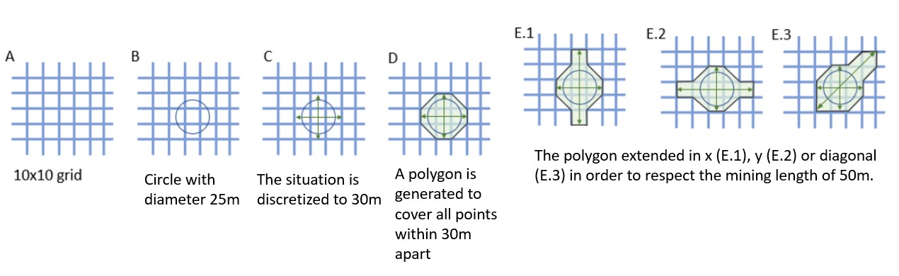
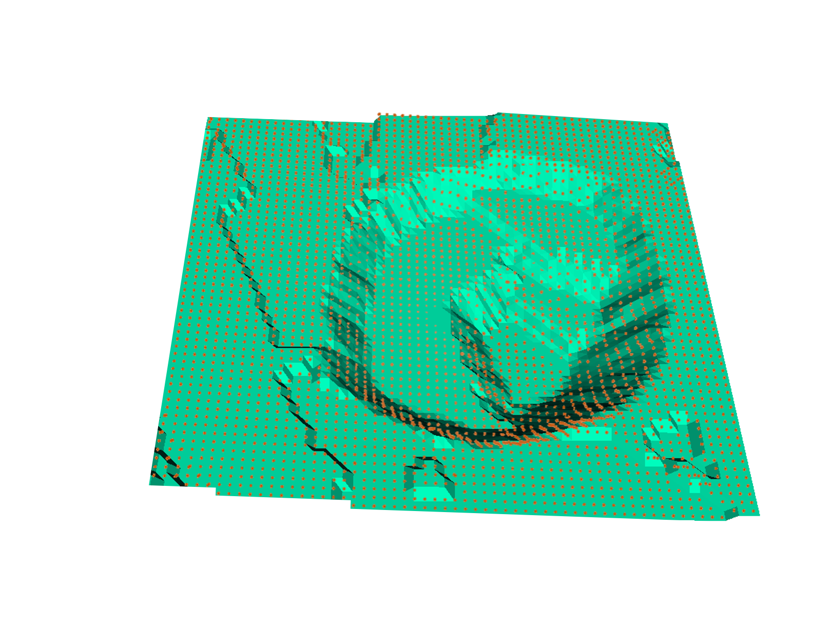


 “The software that could revolutionize mine planning”
 How digital innovation can improve mining productivity
 A tool for these times
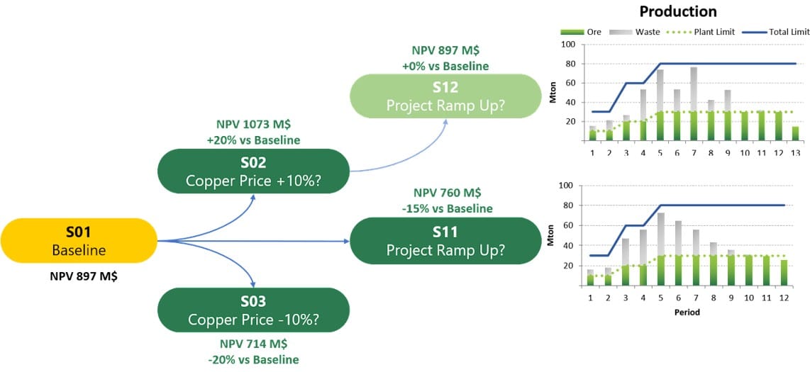
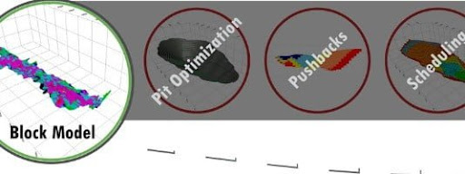
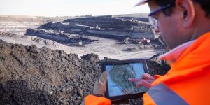 Mine Optimizations and SimSched DBS is a friend of yours now. SimSched DBS is the most powerful tool to achieve and compare NPV results of the pit.