Mining Optimization Algorithm

Estimated reading: 23 minutes 4187 views

MiningMath has a flexible mining optimization algorithm that consists of a Mixed Integer Linear Programming (MILP) formulation and linearization methods that tackle the challenging non-linear aspects of the problem. In addition, MiningMath has its own Branch & Cut algorithm, which provides more efficiency than standard MILP optimizers since it’s fine tuned to this specific optimization problem.

One of the major advantages of MiningMath comes from the mathematical formulations based on surfaces (Goodwin et. al. (2006), Marinho (2013)) instead of usual block precedences. Block precedence methods might lead to higher errors (Beretta and Marinho (2015)), providing slopes steeper (i.e. riskier, more optimistic) than requested. The use of surfaces eliminates these geotechnical errors and allows for block-by-block geotechnical zones, if needed.

Another crucial advantage is that MiningMath’s formulation includes geometric constraints, allowing its algorithm to find solutions that are closer to real mining operations. The user can guide geometries by including mining and bottom widths, maximum vertical advance rates, and forcing/restricting mining areas. Such constraints give freedom to the user to work, or not, with predefined cut-offs and pushbacks which might limit the space of potential solutions. Hence, the software provides different views and solutions for the same mine for each parameter changed.

Eventually, linear solutions need to be mapped onto an approximate integer (block-by-block) solution that will represent the scheduling of the mining problem in the real-world. The intelligence to convert continuous solutions into integer and non-linear ones are made by MiningMath’s Branch & Cut algorithm.

Algorithm’s flowchart and mathematical formulation

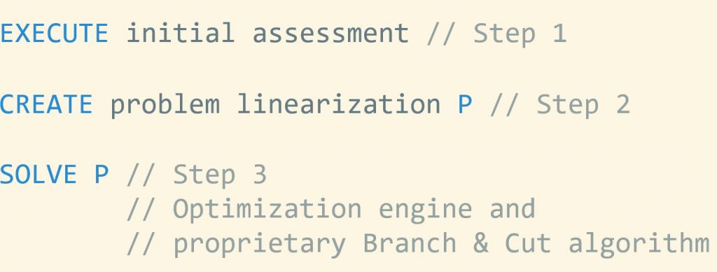
MiningMath employs an innovative mathematical formulation and powerful proprietary Branch & Cut algorithm for mining optimization problems. A description of this mathematical formulation and the three main steps of the algorithm employed are given below.

Step 1: Initial assessment

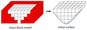
Figure 1: Initial assessment of entire block model and inclusion of likely profitable blocks within an initial surface.

The first step of the mining optimization algorithm is to remove regions that do not add any value to the project. This is an initial assessment that considers slope constraints, reducing the size of the problem and providing a region of interest for the optimization process. Since MiningMath always employs surfaces in its mathematical formulations, this first set of likely profitable blocks are contained within an initial surface as depicted in Figure 1.

Step 2: Problem linearization and mining optimization

In the second step of the mining optimization algorithm, the non-linear, integer problem is approximated to an integer, linear one based on surfaces. For that, it is necessary first to define the common notation across the problem and its variables.

\(S\): number of simulated orebody models considered
\(s\): simulation index, \(s = 1,...,S \)
\(D\): number of destinations
\(d\): destination index, \(d = 1,...,D \)
\(Z\): number of levels in the orebody model
\(z\): level index, \( z = 1,...,Z \)
\(T\): number of periods over which the orebody is being scheduled and also defines the number of surfaces considered
\(t\): period index, \(t = 1,...,T. \)
\(M\): number of cells in each surface; where \(M = x \times y\) represents the number of mining blocks in x and y dimensions.
\(c\): cell index, \(c = 1, \ldots ,M\).
\(G\): number of unique destination groups defined. Each group might contain 1, all, or any combination of destinations.
\(g\): group index, \(g = 1, \ldots ,G\).

\(x_{c,t,d}^{z}\): simulation-independent binary variable that assumes 1 if block \((c, z)\) is being mined in period \(t\) and sent to destination \(d\), and 0 otherwise.
\(e_{c,t}\): simulation-independent continuous variables associated with each cell \(c\) for each period \(t\), representing cell elevations.
\(\overline{f_{t,g,s}},\underline{f_{t,g,s}}\): continuous variables to penalize sum constraints violated for each period, group of destinations, and simulation. One pair of variables is necessary for each quantifiable parameter modeled block by block whose sum is being constrained. An example would be variables used to control fleet hours spent in different periods, groups of destinations, and simulations. More information about possible parameters here. Note also that the software allows the control of the average of simulations, instead of dealing with each simulation individually, and the control by the sum of destinations, instead of each destination individually.
\(\overline{\alpha_{t,g}},\underline{\alpha_{t,g}}\): user defined weights for variables \(\overline{f_{t,g,s}},\underline{f_{t,g,s}}\) with the same destination group \(g\) and period \(t\). These can only be defined in the .ssscn files.
\(\overline{j_{t,g,s}},\underline{j_{t,g,s}}\): continuous variables to penalize average constraints violated for each period, destination, and simulation. One pair of variables is necessary for each quantifiable parameter modeled block by block whose average is being constrained. An example would be variables used to control the average grade of blocks mined in different periods, destination groups, and simulations. More information about possible parameters here. Note also that the software allows the control of the average of simulations, instead of dealing with each simulation individually, and the control by the sum of destinations, instead of each destination individually.
\(\overline{\beta_{t,g}},\underline{\beta_{t,g}}\): user defined weights for variables \(\overline{j_{t,g,s}},\underline{j_{t,g,s}}\) with the same destination \(d\) and period \(t\). These can only be defined in the .ssscn files.

\(e_{c,t} \in \mathbb{R},\,\, \) \(t = 1,...,T\),\(c=1,...,M\)
\(x_{c,t,d}^{z} \in \{0,1\},\,\, \) \(c=1,...,M\), \(t = 1,...,T\), \(z=1,...,Z\), \(d=1,...,D\)
\(\overline{f_{t,d,s}},\underline{f_{t,d,s}} \in \mathbb{R_{\geq 0}}\), \(t = 1,...,T\), \(s=1,...,S\), \(d=1,...,D\)
\(\overline{j_{t,d,s}},\underline{j_{t,d,s}} \in \mathbb{R_{\geq 0}}\), \(t = 1,...,T\), \(s=1,...,S\), \(d=1,...,D\)

Having the set of variables defined, is possible now to define a mathematical model with an objective function and necessary constraints.

Objective function
Intuitive idea
Sum of the economic value of blocks mined per period, destination, and simulation.
Average the result by the number of simulations.
Subtract penalties for certain violated restrictions associated with some user defined parameters.
Requirements
\(V_{c,t,d,s}^{z}\): cumulative discounted economic value of block \((c, z)\) in simulation \(s\), period \(t\) and destination \(d\). More about this calculation here.
Formulation
\(max\frac{1}{s}\)\(\sum\limits_{s=1}^{S}\sum\limits_{t=1}^{T}\sum\limits_{c=1}^{M}\sum\limits_{z=1}^{Z}\sum\limits_{d=1}^{D}\)\((V_{c,t,d,s}^{z} x_{c,t,d}^{z}) \,-\, p\)
where
\(p = \sum\limits_{t=1}^{T}\sum\limits_{g=1}^{G}(\overline{\alpha_{t,g}}(\sum\limits_{s=1}^{S}\overline{f_{t,g,s}})\)\( + \underline{\alpha_{t,g}}(\sum\limits_{s=1}^{S}\underline{f_{t,g,s}})\)\( + \overline{\beta_{t,g}}(\sum\limits_{s=1}^{S}\overline{j_{t,g,s}})\)\( + \underline{\beta_{t,g}}(\sum\limits_{s=1}^{S}\underline{j_{t,g,s}})) \)

Finally, the objective function is constrained by the restrictions below

\(e_{c,t-1} - e_{c,t} \ge 0, c=1,...,M, t=2,...,T \)

Figure 3: Example of crossing surfaces — Figure 3: Two surfaces (blue and yellow): a) not crossing each other and respecting the constraint; b) crossing each other and not respecting the constraint.

Intuitive idea

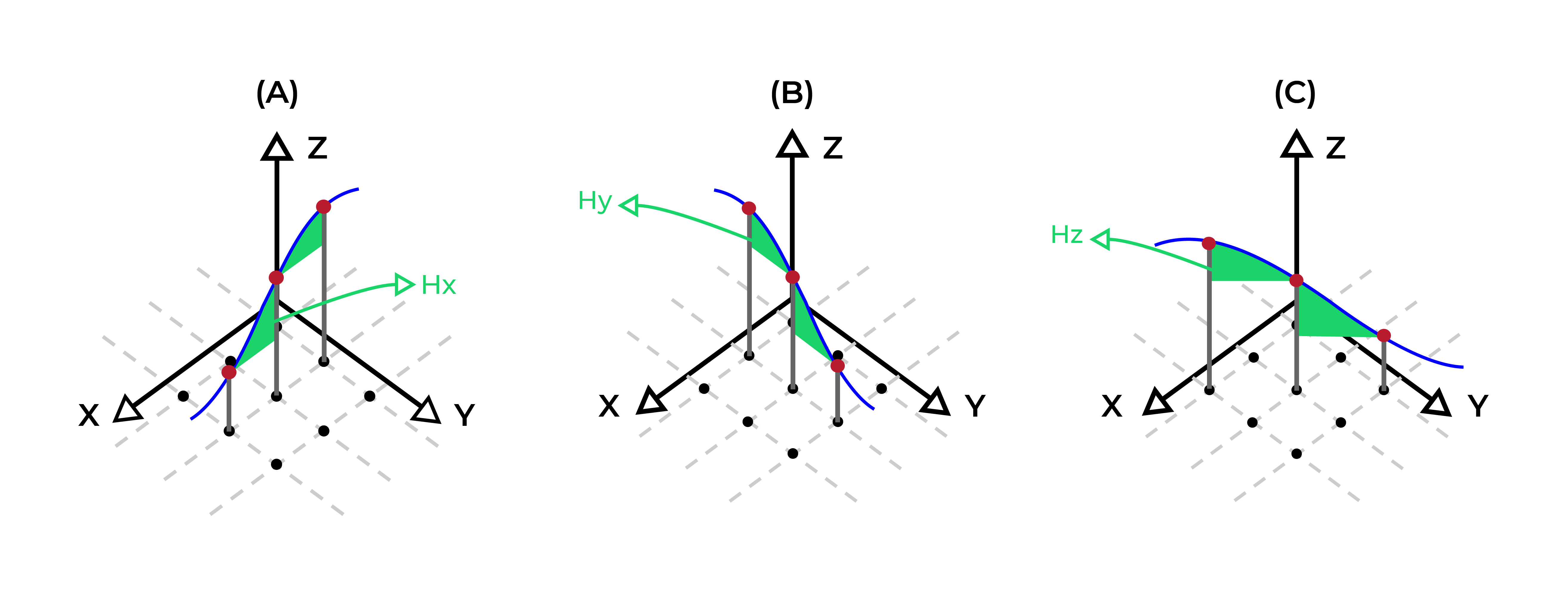
Adjacent elevations in a single surface need to respect a maximum difference. This maximum will change based on which direction they are adjacent: x, y, or diagonally.

Requirements

\(H_x, H_y, H_d\): maximum difference in elevation for adjacent cells in \(x\), \(y\) and diagonal directions
\(X_c, Y_c, D_c\): equivalent to \(H_x, H_y, H_d\)concept, the sets of adjacent cells, laterally in \(x\), in \(y\), and diagonally, for a given cell \(c\), respectively.

Formulation

\(e_{c,t} - e_{x,t} \ge H_x, c=1,...,M, t=1,...,T, x \in X_c\)
\(e_{c,t} - e_{y,t} \ge H_y, c=1,...,M, t=1,...,T, y \in Y_c \)
\(e_{c,t} - e_{d,t} \ge H_d, c=1,...,M, t=1,...,T, d \in D_c \)

Example of slope constraints in mining optimization algoritm — Figure 4: Maximum allowed difference (Hx, Hy, and Hd) in elevation between adjacent cells in contact laterally in the x direction (a), in contact laterally in the y direction (b), and in contact diagonally (c).

Proprietary constraints not disclosed. Possible examples of constraints of the same type, but not the ones actually employed.

Intuitive idea

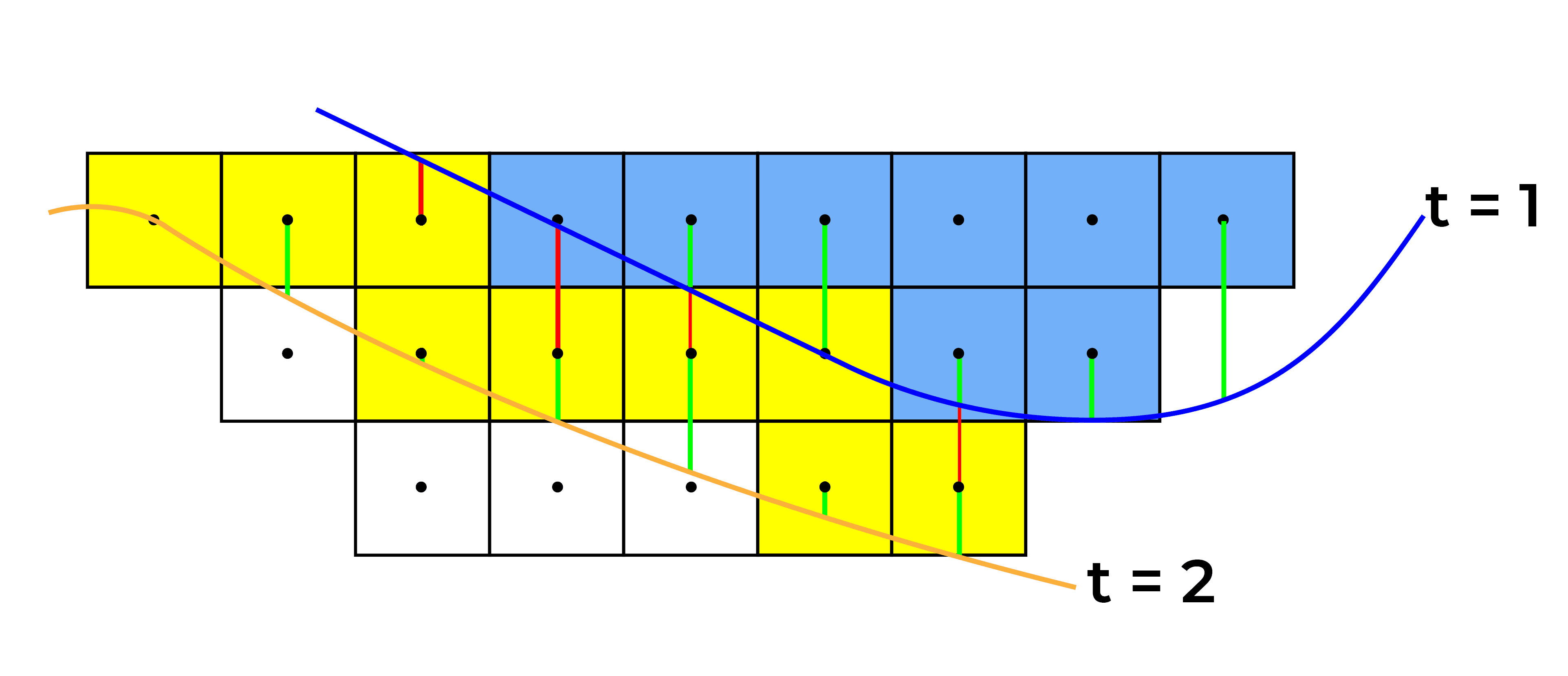
Surfaces will define when blocks will be mined. For example, blocks between surfaces associated with period 1 and 2, will be mined in period two. A block is between two surfaces if its centroid is between the two surfaces.

Requirements

\(E_{c}^{z}\): elevation of centroid for a given block \((c, z)\)

Formulation

\(E_{c}^{z} \times \sum\limits_{d=1}^{D}x_{c,1,d}^{z} \ge e_{c,1}, c=1,...,M, z=1,...,Z\)
\(e_{c,t-1} \ge E_{c}^{z} \times \sum\limits_{d=1}^{D}x_{c,t,d}^{z} \ge e_{c,t}, \)\(c=1,...,M, t=2,...,T, z=1,...,Z\)

Figure 5: Distance between centroids above surfaces (green lines) and below surfaces (red lines) respecting constraints. Blue blocks are mined in period 1, while yellow blocks are mined in period 2.

Intuitive idea

Each mined block can only be sent to one destination.

Formulation

\(\sum\limits_{d =1}^{D}x_{c,t,d}^{z} = 1, c=1,....,M, t=1,...,T, z = 1,...,Z\)

Intuitive idea

For each period and destination groups there’s an upper and lower limit of total tonnage to be extracted. Destination groups might be formed by any unique combination of destinations, with 1, many or all. The sum of the tonnage of mined blocks sent to the same group of destinations in the same period must respect these limits.

Requirements

\(T_c^z\): tonnage for a given block \((c, z)\).
\(\overline{T_{t,g}}\): upper limits in total tonnage to be extracted during period \(t\) and destinations in group \(g\).

Formulation

\( \sum\limits_{c=1}^M\sum\limits_{z=1}^{Z}\sum\limits_{d \in g}T_c^z x_{c,t,d}^{z} \le T_{t,g}, t = 1,...,T, g = 1,..., G\)

Intuitive idea

The user can define a certain parameter (i.e. fleet hours spent) associated with each mined block to have its sum controlled. The sum of the values of this parameter associated to each mined block must respect lower and upper bounds for each period, destination groups (optional) and simulation (individually or on average). Destination groups might be formed by any unique combination of destinations, with 1, many or all.

Requirements

\(\underline{F_{t,g,s}},\overline{F_{t,g,s}}\): lower and upper limits, respectively, in sum of user defined parameter to be respected in period \(t\), destination group \(g\), and simulation \(s\).
\(F_{c,d,s}^{z}\): value of user defined parameter related to a given block \((c, z)\) in destination \(d\) and simulation \(s\).

Formulation

\(\underline{F_{t,g,s}} \le \sum\limits_{c=1}^M\sum\limits_{z=1}^{Z}\sum\limits_{d \in g}F_{c,d,s}^{z}x_{c,t,d}^{z} + \underline{f_{t,g,s}} - \overline{f_{t,g,s}} \le \overline{F_{t,g,s}},\)
\(t = 1,...,T, g = 1,..., G, s = 1,..., S\)

Intuitive idea

The user can define a certain parameter (i.e. grade) associated with each mined block to be controlled in average. This average is weighted by the block’s tonnage and by an optional, user defined weight. It must respect lower and upper bounds for each period, destination group (optional) and simulation (individually or on average). Destination groups might be formed by any unique combination of destinations, with 1, many or all.

Requirements

\(\underline{J_{t,g,s}},\overline{J_{t,g,s}}\): lower and upper limits, respectively, for average value of user defined parameter to be respected in period \(t\), simulation \(s\), and destination group \(g\).
\(T_{c}^{z}\): tonnage for a given block \((c, z)\).
\(J_{c,s,d}^{z}\): value of user defined parameter of block \((c, z)\) sent to destination \(d\) in simulation \(s\)
\(P_{c,t,d,s}^{z}\): user defined weight for block \((c, z)\) in period \(t\), destination \(d\), and simulation \(s\)

Formulation

\(\underline{J_{t,g,s}} \le\)\(\frac{\sum\limits_{c=1}^M\sum\limits_{z=1}^Z\sum\limits_{d\in g}P_{c,t,d,s}^{z}T_{c}^{z}J_{c,s,d}^{z}x_{c,t,d}^{z}}{\sum\limits_{c=1}^M\sum\limits_{z=1}^Z\sum\limits_{d\in g}P_{c,t,d,s}^{z}T_{c}^{z}}\)\( + \underline{j_{t,g,s}} - \overline{j_{t,g,s}} \le \overline{J_{t,g,s}}\)
\(t = 1,...,T, g = 1,..., G, s = 1,..., S\)

Proprietary constraints not disclosed

Intuitive idea

Surfaces should respect geometric parameters defined by the user, such as minimum bottom width, minimum mining width, minimum mining length, and maximum vertical rate of advance, as depicted here.

Formulation

\(Geometric(e_{c,t}) \le \text{geometric restriction}, c=1,...,M, t=1,...,T\)

Step 3: Integer, non-linear solution and evaluation

The next step in the mining optimization algorithm is to convert the linear solution to an integer, non-linear one. MiningMath’s Branch & Cut method is responsible for this conversion. Once it is done, the resulting solution can be evaluated, leading to the end of the algorithm’s execution or to a new optimization process. This new process might be triggered if one of the two situations arise:

restrictions are violated due to transformation from linear to integer, non-linear solution, or due to problem being infeasible.
an evaluation of certain restrictions in the transformed integer, non-linear solution concluded that they might not affect the problem and be better discarded or modified.

If any of these are true, the solution at this stage will be sent back to Step 2 for linearization and refinement. Thus, if this refinement is caused by situation 1) then the goal is to improve the solution’s feasibility. This feasibility is improved according the constraint hierarchy order depicted in Figure 6.

Figure 6: constraints hierarchy order.

In contrast, if it is caused by situation 2) then the goal is to allow the optimization to focus on the bottlenecks of the problem and improve the current NPV. Once none of these situations have been identified, the current solution is returned. Note that each time the algorithm goes back to Step 2, a new global optimization is performed, thus the new resulting solution might be entirely different.

Pseudo-code

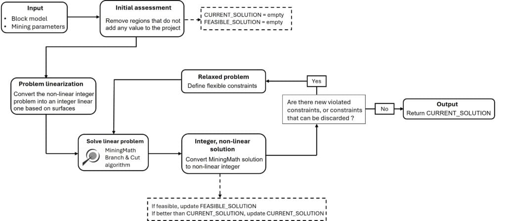
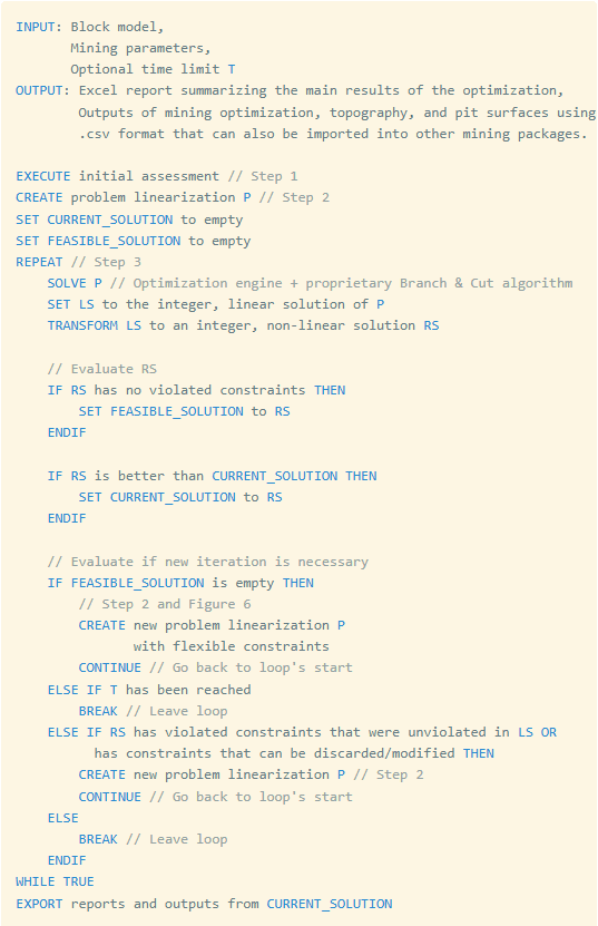
The whole process of the mining optimization algorithm, from input to output is summarized in the psudo-code below. References are made to previous Steps 1, 2, and 3. This algorithmic flow together with the proposed mathematical formulation exemplifies the innovative methodology applied to solve a single mine scheduling problem.

				
					INPUT: Block model,
       Mining parameters,
       Optional time limit T
OUTPUT: Excel report summarizing the main results of the optimization,
        Outputs of mining optimization, topography, and pit surfaces using   
        .csv format that can also be imported into other mining packages.

EXECUTE initial assessment // Step 1
CREATE problem linearization P // Step 2
SET CURRENT_SOLUTION to empty
SET FEASIBLE_SOLUTION to empty
REPEAT // Step 3
    SOLVE P // Optimization engine + proprietary Branch & Cut algorithm
    SET LS to the integer, linear solution of P
    TRANSFORM LS to an integer, non-linear solution RS
    
    // Evaluate RS
    IF RS has no violated constraints THEN
        SET FEASIBLE_SOLUTION to RS
    ENDIF
        
    IF RS is better than CURRENT_SOLUTION THEN 
        SET CURRENT_SOLUTION to RS
    ENDIF
    
    // Evaluate if new iteration is necessary
    IF FEASIBLE_SOLUTION is empty THEN
        // Step 2 and Figure 6
        CREATE new problem linearization P
               with flexible constraints
        CONTINUE // Go back to loop's start
    ELSE IF T has been reached
        BREAK // Leave loop
    ELSE IF RS has violated constraints that were unviolated in LS OR
          has constraints that can be discarded/modified THEN
        CREATE new problem linearization P // Step 2
        CONTINUE // Go back to loop's start
    ELSE
        BREAK // Leave loop
    ENDIF
WHILE TRUE
EXPORT reports and outputs from CURRENT_SOLUTION

MiningMath

Loading...

Mining Optimization Algorithm

Algorithm’s flowchart and mathematical formulation

Step 1: Initial assessment

Step 2: Problem linearization and mining optimization

Objective function

Step 3: Integer, non-linear solution and evaluation

Pseudo-code

CONTENTS

MiningMath

Loading...

Mining Optimization Algorithm

Algorithm’s flowchart and mathematical formulation

Step 1: Initial assessment

Step 2: Problem linearization and mining optimization

Objective function

Surface constraints

Slope constraints

Link constraints

Destination constraints

Mining constraints

Sum constraints

Average constraints

Geometric constraints

Step 3: Integer, non-linear solution and evaluation

Pseudo-code

Mining Optimization Algorithm

CONTENTS