Short-term Planning
Highlights
Integrating short‑term plans with long‑term objectives ensures operations stay aligned to strategic goals as market prices, ore conditions, and equipment availability change.
- Enables simultaneous optimization of both short‑ and long‑term variables, reducing rework and accelerating plan updates—MiningMath’s integrated approach lets engineers iterate scenarios quickly and avoid disjointed schedules.
- Boosts plan adherence and reconciliation, delivering concrete operational consistency—by optimizing with real data, MiningMath helps reconcile daily execution with high-level forecasts .
- Supports automation and API-driven workflows, enabling rapid scenario testing and repeatable updates, a key differentiator compared to manual planning tools.
MiningMath enables the integration between long- and short-term planning, helping you improve plan adherence and reconciliation. It does so by providing custom timeframes for different periods of the project. This page detailes the necessary concepts and their usage withing MiningMath.
Timeframes
Each period in MiningMath can be customized to fit your planning needs, from very short timeframes, such as months, to extended periods spanning decades. For that it employs factors.
Factors
The base factor in MiningMath is 1, which typically represents one year—the most common duration for a planning period. Using 1 as the reference, you can easily define any other timeframe. For example:
- 1/2 as six months
- 1/12 as months
- 3 as trienniuns
- 10 as decades
In the interface, you can set that in the Economics tab, as illustrated below.


Discount rate calculation
The discount rate in MiningMath is defined per year.

When you use custom timeframes, MiningMath automatically adjusts the discount rate internally to match the specified period. For details on how discount rates are calculated for different timeframes, please visit this page.
Integrating long- and short-term planning
Long-term
By running the Super Best Case, you can generate surfaces to guide the optimization based on the NPV upper bound. In turm, the Optimized Pushbacks workflow provides insights on what could be the challenges of your project and also operational designs that could be used in further steps. At last, a detailed Schedule can be obtained by using, or not, a surface, which could be the final pit or any intermediary one, as a guide.
Short-term
Following this long-term workflow, you should now have enough information to build a solid long-term view and improve the adherence and reconciliation of your plans. At this stage, you can select a surface and apply it using Force Mining or Restrict Mining to refine the schedule within its boundaries.
- Force Mining ensures that all material within the selected surface is extracted, while still respecting slope angles.
- Restrict Mining, on the other hand, prevents any material below the defined surface from being mined until the specified period is reached.
This allows MiningMath to precisely reach the defined surface within the chosen timeframe, enabling you to explore different geometries, blending constraints, and other variables required for short-term planning—without compromising the long-term strategy.
Additional tools that can support these refinements include Mining Fronts and Design Enhancement, which allow you to modify surfaces while respecting all constraints and generating results tailored to your needs. Let’s see a more concrete example next.
Example with equal timeframes
Consider the following configuration parameters employing the Marvin dataset.
| Parameters | Value |
|---|---|
Timeframe | Custom factor (0.5) representing semesters. |
Processing capacity | 5 Mt per semester |
Total movement | 20 Mt per semester |
Vertical rate of advance | 60m per semester |
Minimum Mining | 120m |
Bottom width | 100m |
Force and Restrict Mining Surface | Surface for period 5 obtained from the Optimized Pushbacks workflow |
Stockpiling parameters | On |
Play with steeper slope angles in the short term? | Yes |
In MiningMath’s interface, we can check all these inputs in the Overview tab

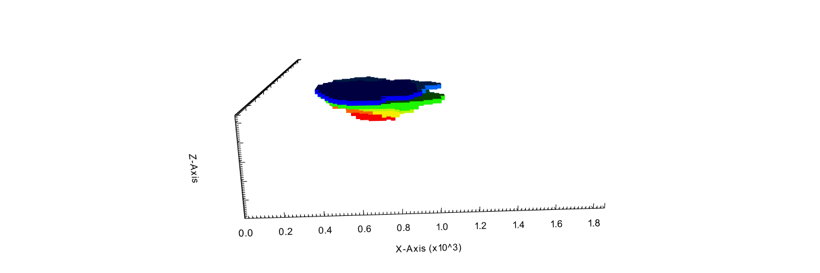
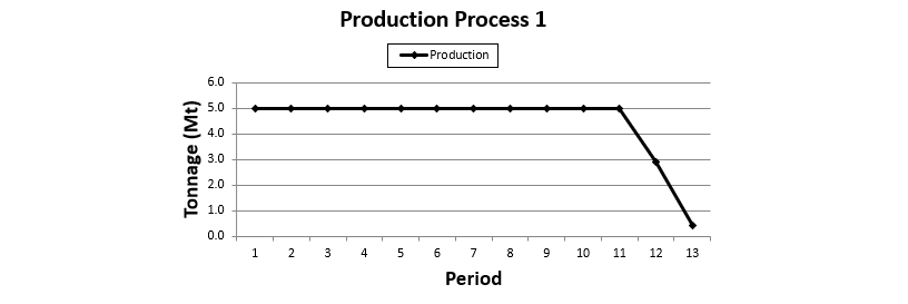
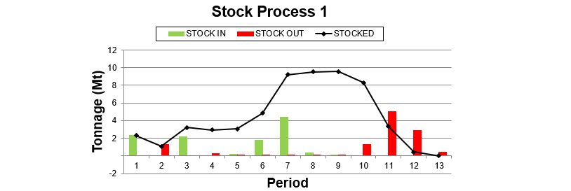
Finally, we can see some of the results after running the scenario illustrated in the images below.
Further details
In the example above, fewer constraints were applied, geometries were adjusted, and the average grade was left unrestricted. Defining the early years with a semester-based timeframe can be especially useful for managing stockpiles and other variables during the first few years—for instance, the initial 3 years of operation.
Keep in mind that period ranges in MiningMath are based on the selected timeframe, so you should adjust your variables accordingly.
When using Force + Restrict Mining, you’re instructing the optimizer to break the specified volume into parts and ensure it is fully mined—even if it contains waste—so that the long-term plan is honored. This lets you maintain a global view of the entire deposit while making more tactical decisions for the initial periods. It’s important to note that Force + Restrict Mining should be used only at the beginning or end of the mine life. Applying these surfaces in intermediate periods may directly interfere with the optimization results.
This approach differs significantly from traditional methods that rely on a series of Revenue Factors through multiple LG/Pseudoflow runs, followed by manual adjustments to define pushbacks without mathematical optimization criteria.
Example with different timeframes
Another strategy is to optimize the short-term along with the long-term using different timeframes. In this approach, the integration between the short and long term visions is made in the same optimization process, facilitating the analysis and strategic definitions.
It is possible to:
- Use shorter timeframes (weeks, months, quarters…) for the early periods of the operation;
- Apply annual timeframes for as long as needed, allowing accurate discounted cash flow calculations;
Define longer periods for the later stages of the mine life, reducing detail where it’s less critical and saving processing time for the early years where precision matters most.
This integrated setup allows for value maximization at the strategic level while ensuring feasibility at the tactical level. It also helps to minimize compliance and reconciliation issues, and improves communication between teams by working from a unified plan.
In this configuration:
- Each period range corresponds to the selected timeframe;
- The discount rate is internally adjusted according to each period’s duration;
- Constraints such as production targets and vertical rate of advance must be aligned with the chosen time intervals.
Example configuration:
- Periods 1 to 6 representing one month each.
- Periods 7 to 12 representing one year each.
- Periods 13 and after representing 10 years each.
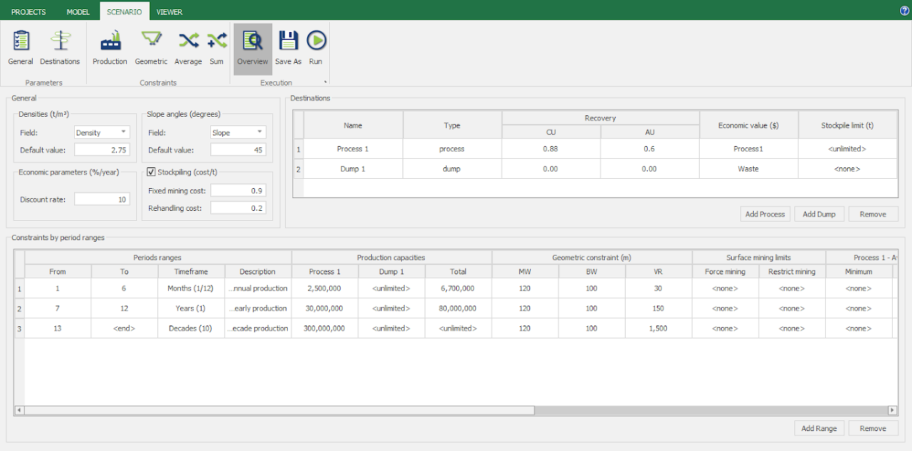
In this case, a 13-period schedule covers 16 years and 6 months, with detailed planning for the first 6 months, yearly breakdowns for the next 6 years, and broader strategic planning for the final decade. The table below illustrates possible parameters for configuring a scenario like this.
| Parameters | Period range 1-6 | Period range 7-12 | Period range 13-end |
|---|---|---|---|
Timeframe | 1/12 of a year (each period representing a month) | 1 year. | 10 years. |
Processing capacity | 2.5 Mt per semester. | 30 Mt per year. | 300 Mt per 10 years. |
Vertical rate of advance | 30m (minimum block size, at this case) per month. | 150m per year. | 1500m per 10 years. |
Minimum Mining | 120m | 120m | 120m |
Bottom Width | 100m | 100m | 100m |
Stockpiling parameters | On | Off | Off |
Different/steeper slope angles in the short term | Yes | No | No |
We can also see the observed inputs in the Overview tab