Mining Fronts
Highlights
Mining fronts define specific zones in the mine plan where constraints can be applied independently, allowing more precise control over production targets and regional strategies. By embedding these controls directly into the model, MiningMath reduces the need for external tools and manual adjustments. This approach supports faster scenario testing and highlights the most profitable areas for mining, aligning operations with both technical and economic goals.
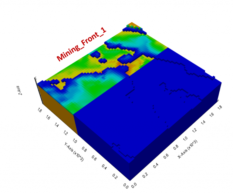
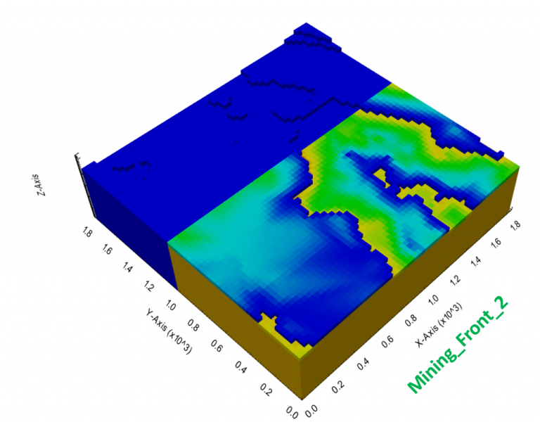
The ‘mining fronts’ approach, as shown in Figure 1 and 2, is a good way to refine results, control regions, and understand which are the best results considering different amounts extracted from a specific place. Using this methodology, you have the possibility to categorize masses by depth, a specific coordinate intervale, even into sectors based on into 360 degrees vision, of your project.
The general idea is pretty similar to what is used to define material types. The first step is to identify the area which you want to control. Then create an additional field regarding the mass on that region and assign it as a sum constraint while importing it. At last, go to the sum tab and control the minimum or maximum amount at the process or dump destinations.
Note that by using this feature you are able to control what, how much, and when the blocks should be mined according to what you want to analyze. This concept is also very useful in the context of mine design, although it increases the complexity while compared with the use of force/restrict mining surfaces, it can also guide solutions, geometrically speaking. It is important to remember that the sum constraint has a high priority parameter in the algorithm and it can also influence the other inputs based on the hierarchy order.
Identify and define your regions as you wish. For instance, use this excel file, place the z from the validation data scenario, calculate the elevation difference with the topography, filter the region which has a 0 result, and create a dispersion chart to identify the final pit. Then, take the coordinates/indexes, which will be the limits of your mining fronts, in this case, the boundary between the mining fronts was at the index 35. Figures 3 and 4 have some visual information to help you.
Calculate the tonnage of your mining front in an additional field and import it as a sum parameter. In this case, the mining front 1 is in the region above or equal to the limit chosen and the mining front 2 is what is bellow it, as seen in Figure 4.
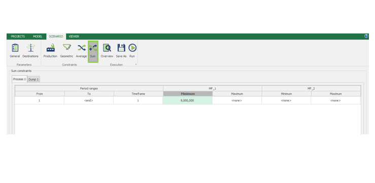
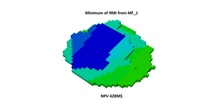
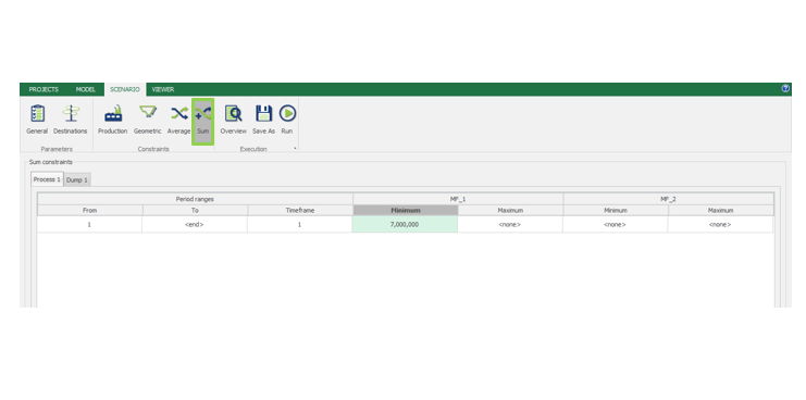
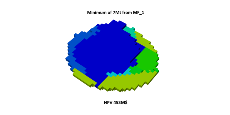
Use the sum tab to control the Mining Front of each destination. Play with the minimum or maximum that should be extracted from each mining front and understand how the results change. The scenarios, that are shown in Figures 5 to 9, used the production, geometric and stockpiling parameters from the Data Validation page.
Download this modified Marvin Deposit file and play on your own.


