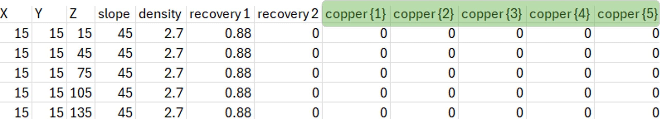
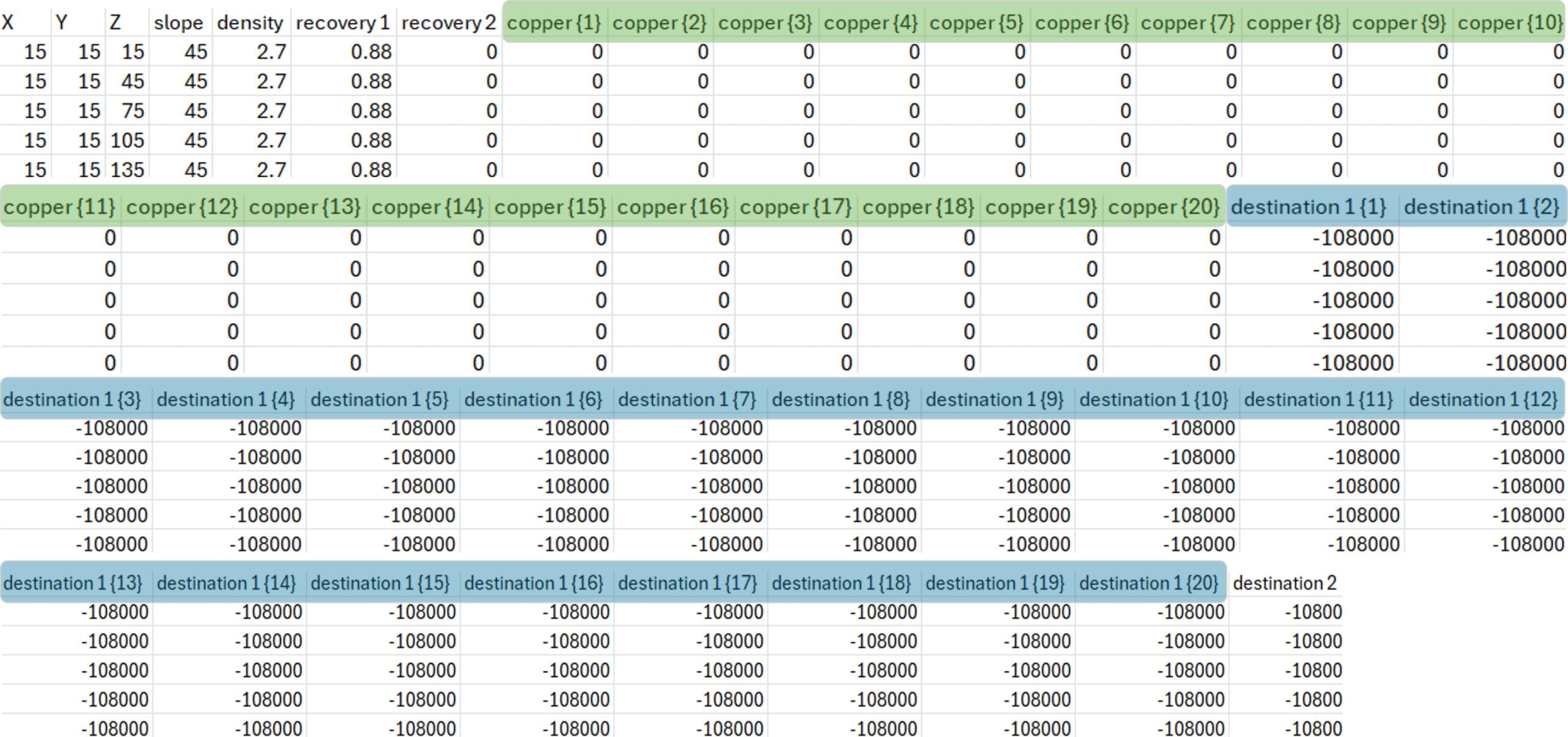
Stochastic Models
While single scenarios of distinct models are run separately, a stochastic scenario consist of obeying all the single scenarios at once. Hence, stochastic simulations requires equiprobable models to consider uncertainties related to geological aspects, such as grade and/or volume of ore. This is achieved through an adapted resource block model that contains equiprobable values for a given set of variables containing a certain level of uncertainty.
As a consequence, MiningMath produces reports with the risk-profile of indicators presenting the minimum, maximum, expected, and percentiles P10 and P90 (these are threshold values, indicating that 10% of the indicators are below the P10 and 90% of the indicators are below the P90). The graphs below illustrate the NPV and cumulative NPV respectively for stochastic models run with MiningMath.

Maximum expected NPV for period 2
Minimum NPV expected for Period 2
P90 NPV for Period 3. 90% of possible expected values for Period 3 are below this point.
P10 NPV for Period 3. 10% of possible expected values for Period 3 are below this point.
Expected NPV for Period 6.

Maximum expected Cumulative NPV for Period 2.
Minimum Cumulative NPV expected for Period 3
P90 Cumulative NPV for Period 4. 90% of possible expected values for Period 3 are below this point.
Expected Cumulative NPV for Period 5.
The purpose of this page is to briefly explain how to import data and manage stochastic constraints using MiningMath.
Formatting Uncertain Fields
Uncertain-fields are those which might vary from simulation to simulation. By definition stochastic models have uncertain fields. Typically, grade fields contain uncertain information. Therefore, the user will need to format each equiprobable possibility in a specific way: name each uncertain column as the same name adding {#} (where # is a number from 1 up to n). The image below highlight how grade headers should look like in a example with 5 simulations.
Note that the grade information will influence the economic values for the processing stream. Therefore, the user will also need to calculate the economic values for each possible grade information, as illustrated below.
Example dataset
The example in this page comes from a simulated copper deposit that can be downloaded here.
Stochastic Constraints
Expected values to control the averages over all simulations.
These constraints will guarantee that, in average, the indicators will be within the defined ranges. For example, take Expected Min = 0.60 and Expected Max = 0.65 for a certain constraint. If there are 3 simulations returning 0.59, 0.62 and 0.65, the average is 0.62, so this is within the range defined.
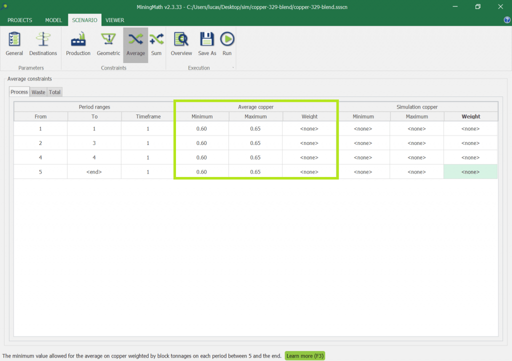
Example to control the average of all simulations. This option is only available when databases containing stochastic data are imported. All simulations to guarantee that each one of them respect certain criteria
These constraints control the variability, or the spread, of the results to be within a certain acceptable range. Let's take an example where such a range has Min = 0.60 and Max = 0.65, and again three simulations returning 0.59, 0.62, and 0.65. In this case the solution will be penalized by the optimizer, as 0.59 < 0.60. Learn more about penalized solutions here.
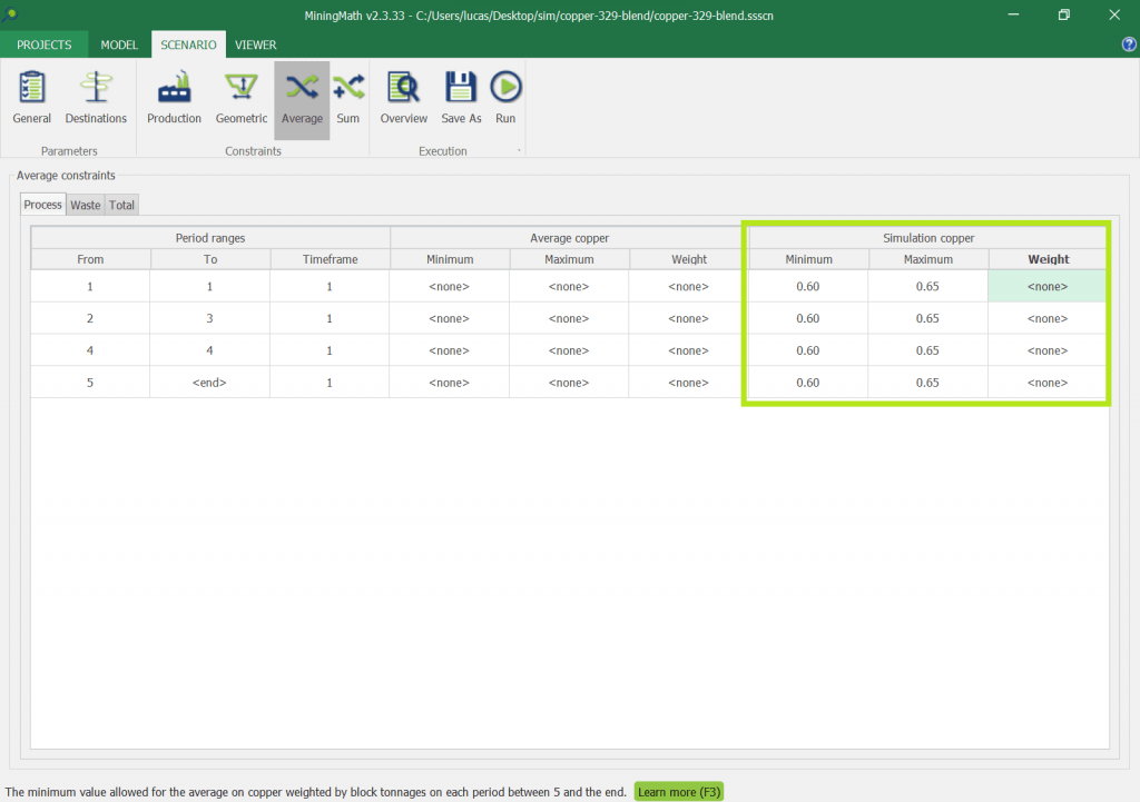
Example to control all simulations individually. This option is only available when databases containing stochastic data are imported.
One schedule
Stochastic optimization is an optimized way to combine all these modelled uncertainties into one schedule that maximizes the expected NPV of the project.
Violated constraints
After executing the optimization with constraints for simulated indicators, it is possible that such constraints will not be respected due to some infeasibility in the problem (more about infeasibilities here).
MiningMath will try to solve any violated constraints following its hierarchy order.
Stochastic constraints are of the average and sum types. They have higher priority than any NPV improvements and time limits imposed by the user.