9. Long-term planning

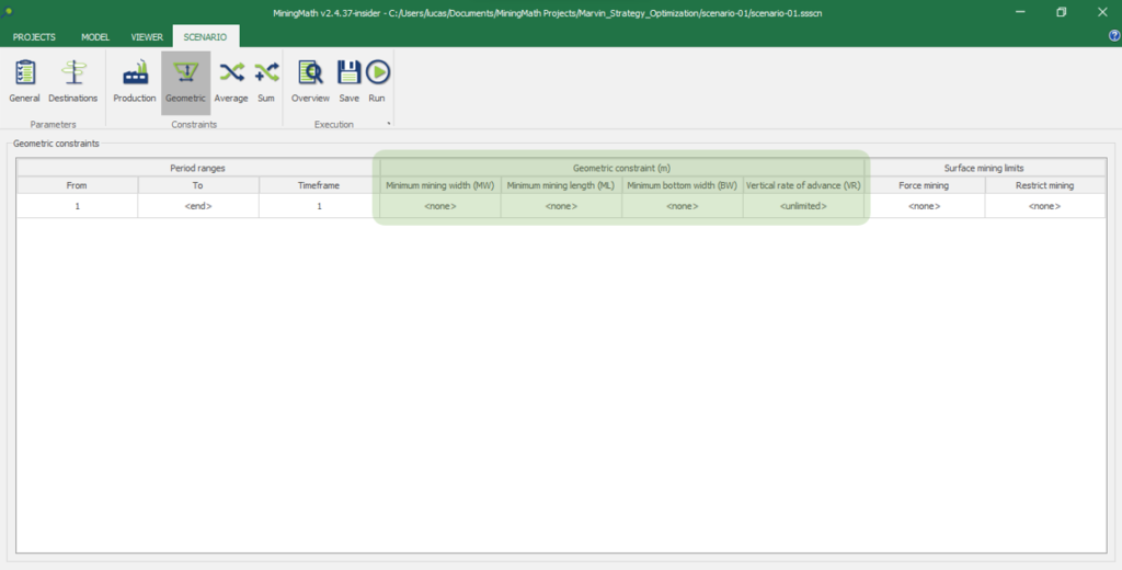
Estimated reading: 4 minutes 162 views

After having refined the NPV upper bound of your project, it is recommended that you start adding geometric constraints. MiningMath incorporates geometric parameters as constraints within the objective function, rather than applying them after pit optimization. This approach enables solutions that align with operational criteria while maximizing net present value (NPV), leading to improved data utilization and identification of opportunities that could be overlooked by manual processes and arbitrary assumptions.

Geometric constraints available

The Geometric tab is the place to set minimum mining & bottom widths, mining length and vertical rate of advance, whose values are applicable to every period.

These parameters are defined as follows:

Mining Width: Distance from a pit to another.

Bottom Width: Bottom minimum area.

Vertical rate of advance: vertical distance mined on each period

Minimum mining length: minimum distance that must exist between at least two points amidst the walls of surfaces among two consecutive mining periods.

Adding a single geometric constraint

When adding more restrictions to a project, it is common for the net present value (NPV) to decrease as the project becomes more restricted. However, since geometric constraints are non linear, it is possible that the results may not follow this trend as new values are tested. To analyze the impact of individual widths or lengths, start by evaluating flexible values to determine an upper bound for NPV under this new geometric constraint, even if the solution is not fully operational yet. Refine these initial results until they are feasible. Assessing geometric constraints is vital for optimizing fleet equipment configuration, maximizing productivity, and increasing project NPV.

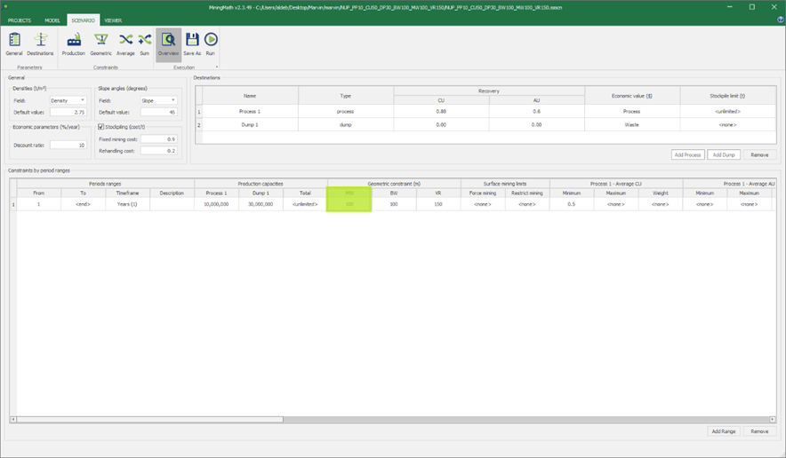
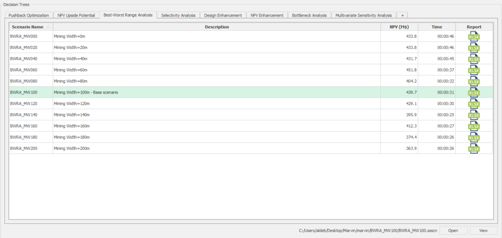
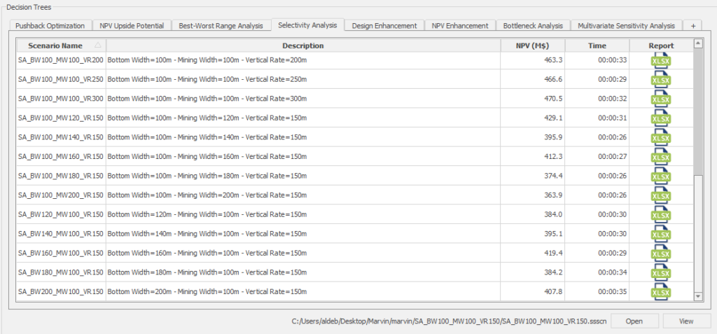
For example, consider the base scenario for the Marvin dataset and subsequent decision tree built to explore different values of mining width.

Evaluation

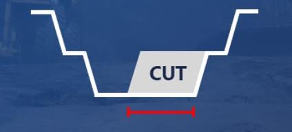
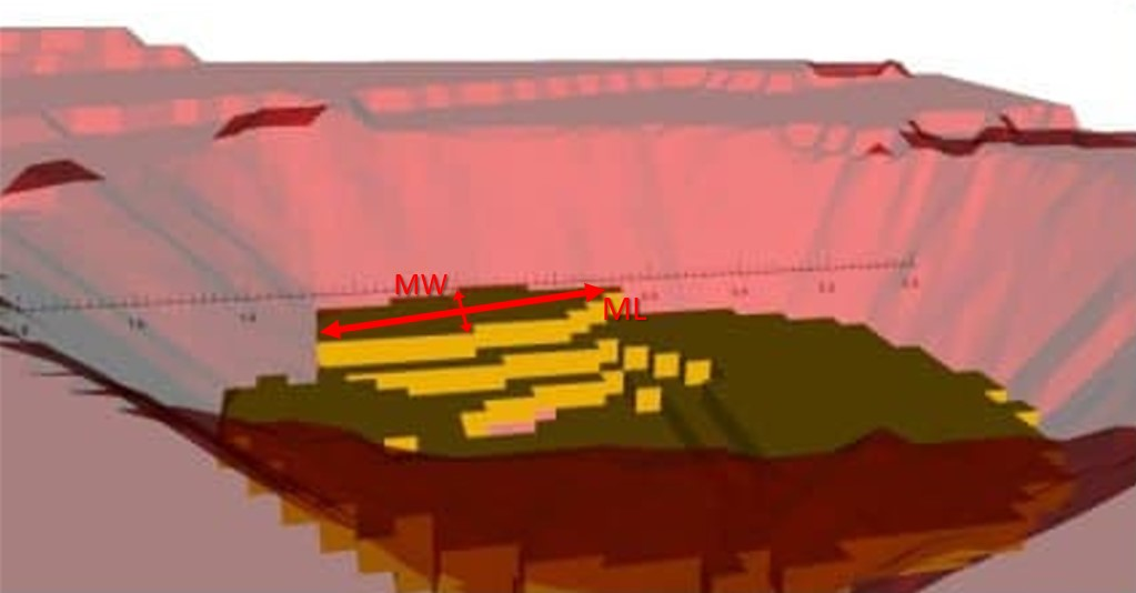
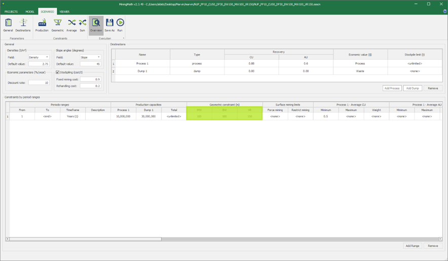
The goal in this case is to understand the impact of different values of mining width (in green), which will be tested with a range of different values, from 0m up to 200m.

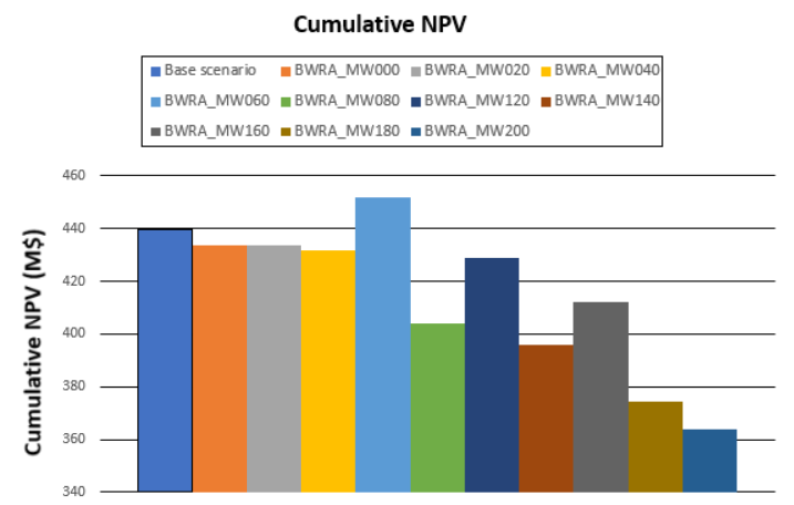
Note that there is no linear relationship between mining width and NPV. In other words, a higher mining width does not necessarily imply a lower NPV. As previously mentioned, that is due to the non-linearity of the problem.

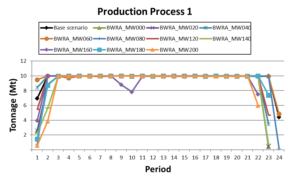
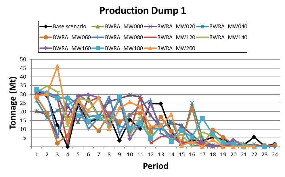
Considering the nature of global optimization employed in MiningMath, other variables might also be affected by different mining widths. For example, the production could be analysed for identification of possible issues when employing different mining widths.

This example illustrates the impact of using different mining widths. However, it could also be reproduced for the other geometric constraints.

Adding multiple geometric constraints

Once you have gained some knowledge on the impact of single geometric constraints, it is important to gain a comprehensive view of the impact of overall geometric limitations on the project’s performance. You can do that by creating scenarios that include each geometric constraint sequentially and gradually increasing or decreasing their values from the least selective until the desirable requirement.

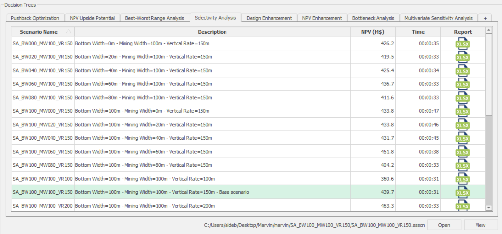
Consider the following base scenario and decision tree built to investigate the use of bottom width, mining width and vertical rate of advance using the Marvin dataset.

Evaluation

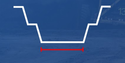
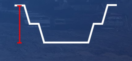
The goal is to understand the impact of different values of geometric constraints. The geometric parameters (in green) will be tested with a range of different values: bottom width with values from 0m up to 200m; mining width with values from 0m up to 200m; and vertical rate of advance with values from 50m up to 300m. In this example, 26 different scenarios were evaluated.

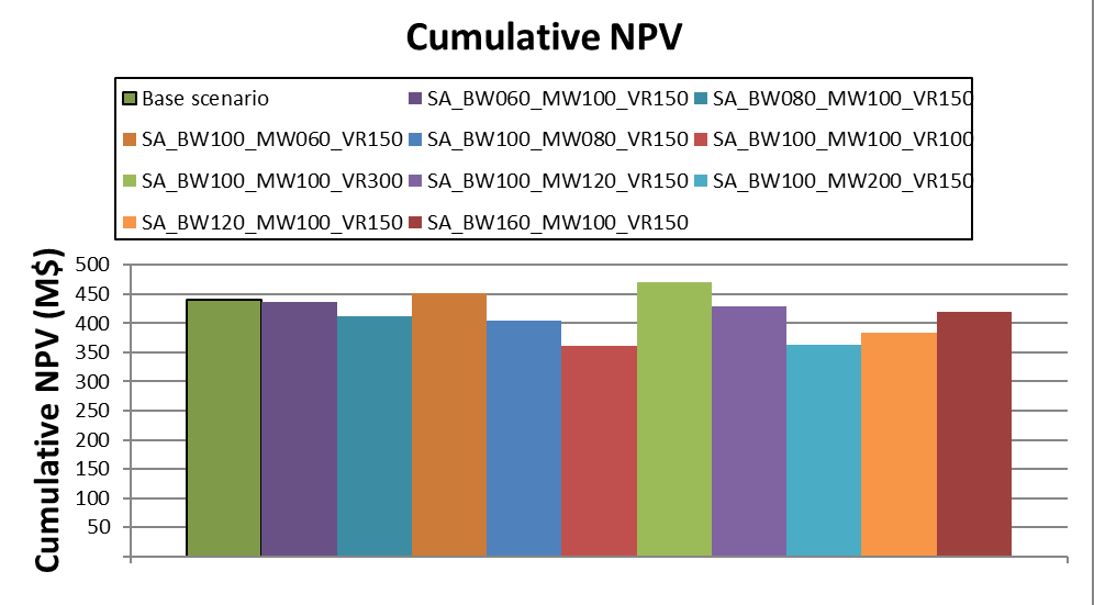
Note that there is no linear relationship between geometric constraints and NPV. In other words, a higher width or lower vertical rate of advance do not necessarily imply a lower NPV. As previously mentioned, that is due to the non-linearity of the problem. The cumulative NPV of the scenarios is compared in the graph below.

There are usually two outcomes when performing such an analysis:

Contrasting geometrics parameters with small NPV variations; or
Similar geometric parameters with larger NPV variations.

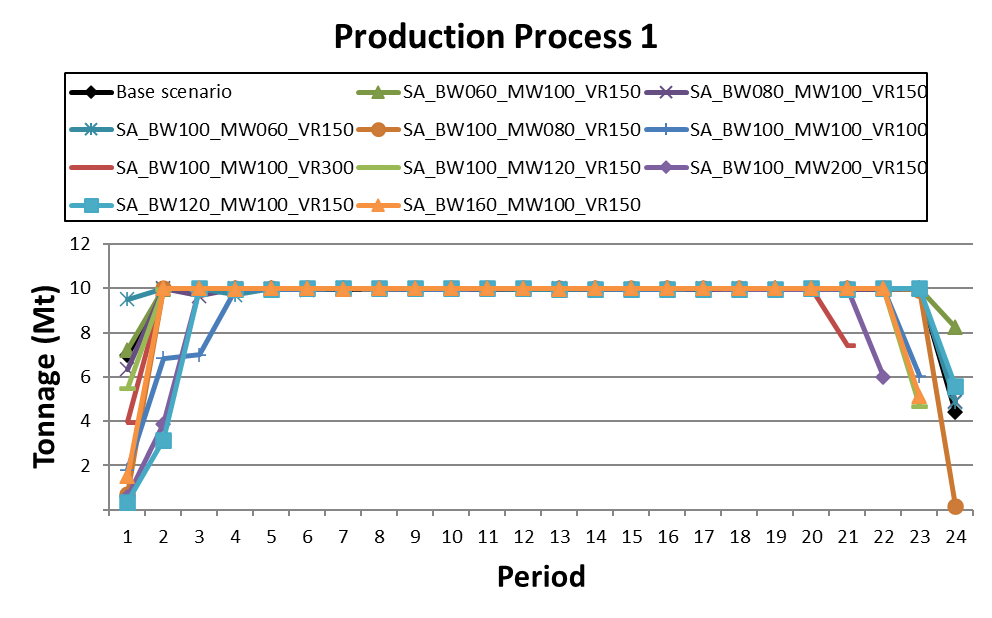
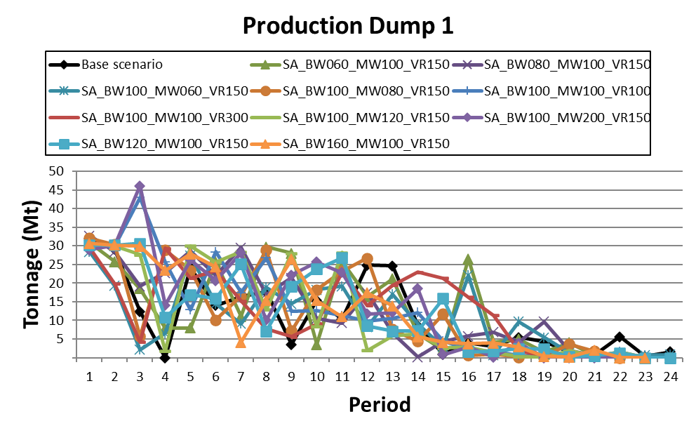
In conclusion, it is important to create several scenarios to perform your long term planning. As exemplified above, results can be quite similar or quite different due to the non-linearity of the problem. Considering the nature of global optimization employed in MiningMath, it is also important to evaluate other indicators. The figures below depict the tonnage achieved for the production, demonstrating the possible impacts for different geometric constraints.

Conclusion

At this stage you should be familiar with the most basic concepts in MiningMath. This will give you the skills to start working on your own data. Each project is different, and might require different analysis and adjustments. You can see other type of common analyses performed with MiningMath here. Also, you can check a suggestion of pages for more advanced concepts here.

MiningMath

Loading...

9. Long-term planning

Geometric constraints available

Adding a single geometric constraint

Evaluation

Adding multiple geometric constraints

Evaluation

Conclusion

CONTENTS